Plot with Makie

This site draws with Plots.jl by default. Makie.jl is the second backend, at feature parity — same figures, same keywords. The one real difference is how you call it, and that difference is worth a page of its own.

When to use it

Stay on Plots unless one of these is true: you want an interactive window to pan and zoom into a switching time or a stiff region, or you are already drawing in Makie elsewhere in your project and want one plotting stack, not two.

Loading a backend

CairoMakie

using CairoMakie   # static — what this page uses

GLMakie

using GLMakie   # interactive — a window you can pan and zoom

Qualify plot

OptimalControl re-exports Plots' plot/plot!. Loading a Makie backend brings in its plot/plot! too — same names, different functions — so the bare call becomes ambiguous:

using OptimalControl
using NLPModelsIpopt
using CairoMakie

julia> plot
UndefVarError: `plot` not defined in `Main`
Hint: It looks like two or more modules export different bindings with this name, resulting in ambiguity. Try explicitly importing it from a particular module, or qualifying the name with the module it should come from.
Hint: a global variable of this name also exists in GR.jlgr.
    - Also exported by GR.
Hint: a global variable of this name also exists in RecipesBase.
    - Also exported by OptimalControl.
    - Also exported by Plots.
Hint: a global variable of this name also exists in Makie.
    - Also exported by CairoMakie.

Julia's own hint names both modules. The fix is to always qualify the Makie call:

Makie.plot(sol)    
Makie.plot(sol)    

Everything else is untouched — solve, state, control, costate, objective, time_grid, Flow, @def all resolve exactly as before. plot and plot! are the only two names that collide.

The same figures

t0 = 0
tf = 1
x0 = [-1, 0]
xf = [0, 0]

ocp = @def begin
    t ∈ [t0, tf], time
    x ∈ R², state
    u ∈ R, control
    x(t0) == x0
    x(tf) == xf
    ẋ(t) == [x₂(t), u(t)]
    ∫(0.5u(t)^2) → min
end

sol = solve(ocp; display=false)

Makie.plot(sol)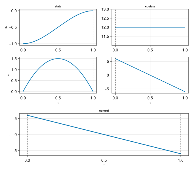

Makie.plot(sol; layout=:group, control=:all)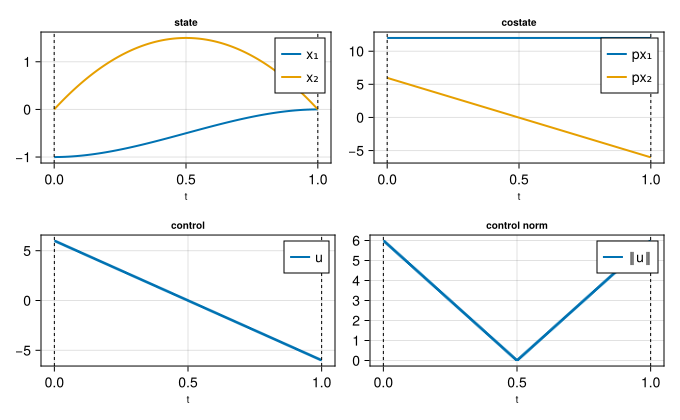

A problem with a box control constraint and a path constraint, the same one used on Plot:

ocp_c = @def begin
    tf ∈ R, variable
    t ∈ [0, tf], time
    x = (q, v) ∈ R², state
    u ∈ R, control
    tf ≥ 0
    -1 ≤ u(t) ≤ 1
    q(0) == -1
    v(0) == 0
    q(tf) == 0
    v(tf) == 0
    1 ≤ v(t) + 1 ≤ 1.8, (c1)
    ẋ(t) == [v(t), u(t)]
    tf → min
end
sol_c = solve(ocp_c; display=false)
Makie.plot(sol_c, :state, :costate, :control, :path, :dual)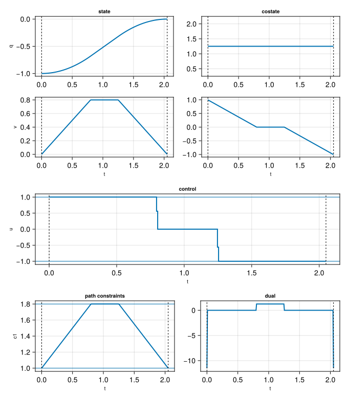

Every keyword documented on Plot — layout, control, time, the *_style/*_bounds_style keywords, size, plot! for overlay — works here unchanged. Only the call itself, and how you customise beyond it, differ.

What differs

	Plots	Makie
the call	plot(sol)	Makie.plot(sol) — always qualified
returns	Plots.Plot	Makie.Figure
reaching one panel	plt[i]	f.content[i] (an Axis)
annotating a panel	Plots.plot!(plt[i], …), hline!	lines!(ax, …), hlines!, text!
*_style contents	any Plots attribute	Makie attributes only — an unknown one throws
a solution into an axis you built	plot!(plt[i], sol)	not supported — Makie.plot! is figure-level (see below)

The *_style keywords hold backend attributes, not a shared vocabulary — a Plots-only name raises instead of being silently dropped:

julia> Makie.plot(sol, :state; state_style=(markershape=:circle,))
Invalid attribute markershape for plot type Makie.Lines{Tuple{Vector{GeometryBasics.Point{2, Float64}}}}.

The available plot attributes for Makie.Lines{Tuple{Vector{GeometryBasics.Point{2, Float64}}}} are:

alpha        cycle            inspector_hover  lowclip      ssao          
clip_planes  depth_shift      inspector_label  miter_limit  transformation
color        fxaa             joinstyle        model        transparency  
colormap     highclip         linecap          nan_color    visible       
colorrange   inspectable      linestyle        overdraw                   
colorscale   inspector_clear  linewidth        space

Annotating the figure

plot/plot! build a whole figure in one call — a convenience on top of the backend, not the backend itself. To add something of your own, reach into the figure and use Makie directly. A time-minimal problem makes this concrete: mark the control bounds and the switching time.

ocp_bb = @def begin
    tf ∈ R, variable
    t ∈ [0, tf], time
    x ∈ R², state
    u ∈ R, control
    tf ≥ 0
    -1 ≤ u(t) ≤ 1
    x(0) == [0, 1]
    x(tf) == [0, 0]
    ẋ(t) == [x₂(t), u(t)]
    tf → min
end
sol_bb = solve(ocp_bb; display=false)

f = Makie.plot(sol_bb, :state, :control)
ax = f.content[3]   # the control panel — see "Where the panels are" below
f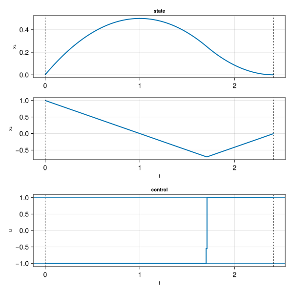

Makie.hlines!(ax, [-1.0, 1.0]; color=:red, linestyle=:dash)
tf_bb = variable(sol_bb)
Makie.vlines!(ax, [tf_bb / 2]; color=:green)
Makie.text!(ax, tf_bb / 2, 0.0; text="switch")
f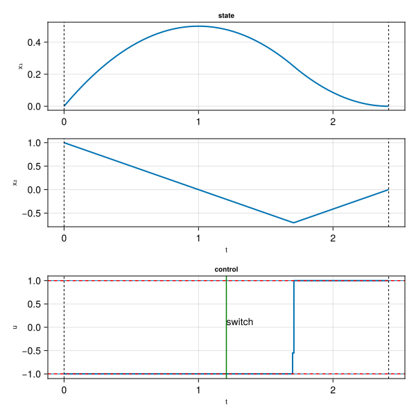

Two calls do the annotating here, and they are not interchangeable:

• Makie.plot!(f, sol) overlays another solution onto the whole figure — the CT extension, Figure-level, the Makie counterpart of Plots.plot!(plt, sol2).

• hlines!(ax, …), vlines!(ax, …), lines!(ax, …), text!(ax, …) add native Makie series onto one panel — plain Makie, Axis-level.

On Plots, plot! does both jobs — overlay a solution and add a native series, the same function either way — which is why a reader coming from Plots reaches for Makie.plot!(ax, sol) here. It fails:

julia> Makie.plot!(ax, sol_bb)
No recipe for plot with args: Tuple{CTModels.Solutions.Solution{CTModels.Solutions.UnifiedTimeGridModel{Vector{Float64}}, CTModels.Components.TimesModel{CTModels.Components.FixedTimeModel{Int64}, CTModels.Components.FreeTimeModel}, CTModels.Components.StateModelSolution{CTModels.Components.CoercedTrajectory{CTBase.Interpolation.Interpolant{CTBase.Interpolation.Linear, Vector{Float64}, Vector{Vector{Float64}}}, typeof(identity)}}, CTModels.Components.ControlModelSolution{CTModels.Components.CoercedTrajectory{CTBase.Interpolation.Interpolant{CTBase.Interpolation.Constant, Vector{Float64}, Vector{Vector{Float64}}}, typeof(only)}}, CTModels.Components.VariableModelSolution{Float64}, CTModels.Models.Model{CTBase.Traits.Autonomous, CTModels.Components.TimesModel{CTModels.Components.FixedTimeModel{Int64}, CTModels.Components.FreeTimeModel}, CTModels.Components.StateModel, CTModels.Components.ControlModel, CTModels.Components.VariableModel, Main.var"#fun##13146#163", CTModels.Components.MayerObjectiveModel{Main.var"#fun##13148#164"}, CTModels.Components.ConstraintsModel{Tuple{Vector{Float64}, CTModels.Building.CompositeConstraint{:path, Tuple{}}, Vector{Float64}, Vector{Symbol}}, Tuple{Vector{Float64}, CTModels.Building.CompositeConstraint{:boundary, Tuple{Main.var"#fun##13133#161", Main.var"#fun##13139#162"}}, Vector{Float64}, Vector{Symbol}}, Tuple{Vector{Float64}, Vector{Int64}, Vector{Float64}, Vector{Symbol}, Vector{Vector{Symbol}}}, Tuple{Vector{Float64}, Vector{Int64}, Vector{Float64}, Vector{Symbol}, Vector{Vector{Symbol}}}, Tuple{Vector{Float64}, Vector{Int64}, Vector{Float64}, Vector{Symbol}, Vector{Vector{Symbol}}}}, CTModels.Components.Definition, Main.var"#165#166"}, CTModels.Components.CoercedTrajectory{CTBase.Interpolation.Interpolant{CTBase.Interpolation.Linear, Vector{Float64}, Vector{Vector{Float64}}}, typeof(identity)}, Float64, CTModels.Solutions.DualModel{CTModels.Components.CoercedTrajectory{CTBase.Interpolation.Interpolant{CTBase.Interpolation.Linear, Vector{Float64}, Vector{Vector{Float64}}}, typeof(identity)}, Vector{Float64}, CTModels.Components.CoercedTrajectory{CTBase.Interpolation.Interpolant{CTBase.Interpolation.Linear, Vector{Float64}, Vector{Vector{Float64}}}, typeof(identity)}, CTModels.Components.CoercedTrajectory{CTBase.Interpolation.Interpolant{CTBase.Interpolation.Linear, Vector{Float64}, Vector{Vector{Float64}}}, typeof(identity)}, CTModels.Components.CoercedTrajectory{CTBase.Interpolation.Interpolant{CTBase.Interpolation.Constant, Vector{Float64}, Vector{Vector{Float64}}}, typeof(only)}, CTModels.Components.CoercedTrajectory{CTBase.Interpolation.Interpolant{CTBase.Interpolation.Constant, Vector{Float64}, Vector{Vector{Float64}}}, typeof(only)}, Float64, Float64}, CTModels.Solutions.SolverInfos{Any, Dict{Symbol, Any}}}}

Makie.plot!(ax, sol_bb)                    
Makie.lines!(ax, time_grid(sol_bb), …)     

Use the native call instead — lines!, hlines!, scatter!, text! — for anything you draw yourself.

Where the panels are

Each panel is an Axis, in the order the description symbols were given, and it carries the component's label — so you can check you grabbed the right one instead of counting:

[(title=string(ax.title[]), ylabel=string(ax.ylabel[])) for ax in f.content]

3-element Vector{@NamedTuple{title::String, ylabel::String}}:
 (title = "state", ylabel = "x₁")
 (title = "", ylabel = "x₂")
 (title = "control", ylabel = "u")

Same ordering Plot documents for plt[i].

Building a figure from scratch

When annotating an existing panel is not enough — a custom layout, a different kind of plot entirely — draw straight from the accessors instead of going through plot at all:

using LinearAlgebra
tg = time_grid(sol_bb)
u = control(sol_bb)

fig = Figure(size=(500, 300))
axu = Axis(fig[1, 1]; xlabel="t", ylabel="‖u‖")
Makie.lines!(axu, tg, norm.(u.(tg)))
fig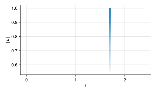

The logo builds a whole figure this way, orbit trajectories and all — the worked example for this approach.

Interactive plots

GLMakie opens a real window instead of rendering to an image — useful to pan and zoom into a switching structure. It cannot run inside this site's own (headless) build, so this block is illustrative only:

using GLMakie

f = Makie.plot(sol)   # opens a window; unaffected otherwise

Flows

The same call works on a trajectory produced by Flow — see Flows for how to build one:

using OrdinaryDiffEqTsit5

p = costate(sol)
p0 = p(t0)
flow = Flow(ocp, (x, p) -> p[2])
sol_flow = flow((t0, tf), x0, p0)
Makie.plot(sol_flow)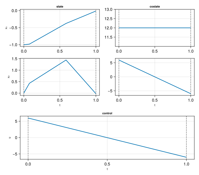

Reference

Makie.plot Method

plot(
    sol::CTModels.Solutions.Solution,
    description::Symbol...;
    kwargs...
) -> Makie.Figure

Plot the components of an optimal control CTModels.Solutions.Solution with a Makie backend.

Same description and keyword arguments as the Plots-backend plot (layout, control, time, the *_style / *_bounds_style keywords, color, size). Returns a Makie.Figure.

Example

julia> using CairoMakie

julia> plot(sol)

julia> plot(sol, :state, :control; layout=:group, control=:all)

Makie.plot! Method

plot!(
    f::Makie.Figure,
    sol::CTModels.Solutions.Solution,
    description::Symbol...;
    kwargs...
) -> Makie.Figure

Overlay the optimal control solution sol onto the existing Makie.Figure f. Same behaviour and keyword arguments as the Plots-backend plot; an empty f is filled as if by plot.

See also

• Plot — the Plots backend and the full keyword reference; every keyword there applies here too.

• The logo — a whole figure built from the accessors, Makie throughout.

• Flows — building the Flow used in the last section.