
Singular control
A vehicle in the plane with drift, time-optimal, whose extremal control is neither
For the minimal case, where the singular control drops out of the optimality conditions with no brackets at all, see Turnpike (bang–singular–bang) first.
using OptimalControl
using NLPModelsIpopt
using OrdinaryDiffEqTsit5
using NonlinearSolve
using Plots
The problem
State
Definition
ocp = @def begin
    tf ∈ R, variable
    t ∈ [0, tf], time
    q = (x, y, θ) ∈ R³, state
    u ∈ R, control

    -1 ≤ u(t) ≤ 1
    -π / 2 ≤ θ(t) ≤ π / 2   # helps direct convergence

    x(0) == 0
    y(0) == 0
    x(tf) == 1
    y(tf) == 0

    ∂(q)(t) == [cos(θ(t)), sin(θ(t)) + x(t), u(t)]

    tf → min
end
Abstract definition:
tf ∈ R, variable
t ∈ [0, tf], time
q = ((x, y, θ) ∈ R³, state)
u ∈ R, control
-1 ≤ u(t) ≤ 1
-π / 2 ≤ θ(t) ≤ π / 2
x(0) == 0
y(0) == 0
x(tf) == 1
y(tf) == 0
(∂(q))(t) == [cos(θ(t)), sin(θ(t)) + x(t), u(t)]
tf → min
The (autonomous) optimal control problem is of the form:
minimize J(q, u, tf) = g(q(0), q(tf), tf)
subject to
q̇(t) = f(q(t), u(t), tf), t in [0, tf] a.e.,
ϕ₋ ≤ ϕ(q(0), q(tf), tf) ≤ ϕ₊,
x₋ ≤ q(t) ≤ x₊,
u₋ ≤ u(t) ≤ u₊,
where q(t) = (x(t), y(t), θ(t)) ∈ R³, u(t) ∈ R and tf ∈ R.The
Direct solution
direct_sol = solve(ocp; grid_size=50, display=false)
plt = plot(direct_sol, :state, :control; label="Direct")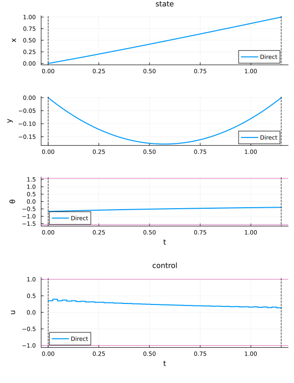
Computing the singular control
The pseudo-Hamiltonian
Splitting the dynamics into a drift and a control vector field,
F0(q) = [cos(q[3]), sin(q[3]) + q[1], 0]
F1(q) = [0, 0, 1]
F1 (generic function with 1 method)H0 = Lift(F0)
H1 = Lift(F1)
H01 = @Lie {H0, H1}
H001 = @Lie {H0, H01}
H101 = @Lie {H1, H01}
us_bracket(q, p) = -H001(q, p) / H101(q, p)us_bracket (generic function with 1 method)The classical singular-control formula
u_indirect(x) = sin(x[3])^2u_indirect (generic function with 1 method)This is exact on the singular surface
q_s = [0.3, -0.1, 0.5]
p_s = [1.7, 1.7 * tan(q_s[3]), 0.0]      # a point of {H₁ = 0, H₀₁ = 0}

us_bracket(q_s, p_s), u_indirect(q_s)    # equal
(0.22984884706593012, 0.22984884706593015)Indirect solution
f = Flow(ocp, (x, p, v) -> u_indirect(x))OptimalControlFlow
├─ system: HamiltonianSystem
│ ├─ time_dependence: Autonomous
│ ├─ variable_dependence: NonFixed
│ ├─ ComposedHamiltonian: autonomous, variable
│ │ natural call: h(x, p, v)
│ │ uniform call: h(t, x, p, v)
│ └─ backend: DifferentiationInterface{CPU}(ad_backend=AutoForwardDiff)
└─ integrator: SciML{CPU} (instance, id=:sciml)
├─ internalnorm = real_norm [default]
├─ alg = Tsit5 [default]
├─ reltol = 1.0e-8 [default]
├─ save_everystep = auto [default]
├─ abstol = 1.0e-8 [default]
├─ save_start = auto [default]
└─ dense = auto [default]
Tip: use describe(SciML{CPU}) to see all available options.Unknowns: the initial costate
t0 = 0

function shoot!(s, ξ)
    p0, θ0, tf = ξ[1:3], ξ[4], ξ[5]

    q_t0 = [0, 0, θ0]
    q_tf, p_tf = f(t0, q_t0, p0, tf; variable=tf)

    s[1] = q_tf[1] - 1
    s[2] = q_tf[2]
    s[3] = p0[3]
    s[4] = p_tf[3]

    px_tf, py_tf, θf = p_tf[1], p_tf[2], q_tf[3]
    s[5] = px_tf * cos(θf) + py_tf * (sin(θf) + 1) - 1
    return nothing
end
shoot! (generic function with 1 method)nle!(s, ξ, _) = shoot!(s, ξ)
p0_guess = costate(direct_sol)(t0)
θ0_guess = state(direct_sol)(t0)[3]
tf_guess = variable(direct_sol)
ξ_guess = [p0_guess..., θ0_guess, tf_guess]
prob = NonlinearProblem(nle!, ξ_guess)
shooting_sol = NonlinearSolve.solve(prob; show_trace=Val(false))
p0_sol, θ0_sol, tf_sol =
shooting_sol.u[1:3], shooting_sol.u[4], shooting_sol.u[5]([0.7826328346326092, -0.6224836112084414, 0.0], -0.6719121189244027, 1.149730885756096)s = zeros(5)
shoot!(s, shooting_sol.u)
s5-element Vector{Float64}:
-7.771561172376096e-16
8.926311769960313e-18
0.0
-1.9524725138148283e-13
-1.346700528870315e-13Comparison
indirect_sol = f((t0, tf_sol), [0, 0, θ0_sol], p0_sol; variable=tf_sol)
plot!(
    plt, indirect_sol, :state, :control;
    label="Indirect", linestyle=:dash,
)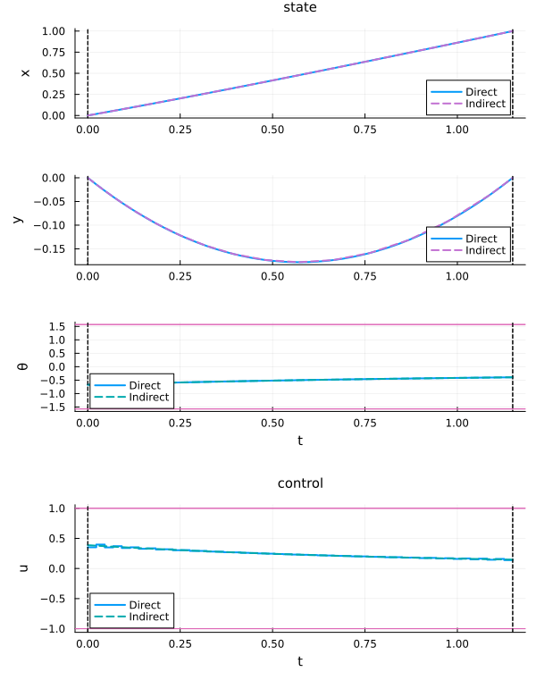
The indirect and direct solutions match closely, confirming the singular-control computation above is correct — and, since Lift/@Lie needed no change from the pre-rewrite version, that the flow half was migrated correctly too.
The same equality, now along the computed extremal rather than a hand-picked surface point:
xs = state(indirect_sol)
ps = costate(indirect_sol)
[us_bracket(xs(t), ps(t)) - u_indirect(xs(t))
 for t in range(t0, tf_sol, 5)]
5-element Vector{Float64}:
2.927402764640874e-11
2.0201063044567036e-11
1.715261266355128e-11
-1.507077795892542e-11
-9.912654030941326e-12See also
Poisson bracket — the
/ / chain, in general. The
@Liemacro — the{}bracket notation used above.Lifting a vector field —
Lift, in general.Shooting — the shooting method in general.