State constraint

The double integrator again, this time with a state constraint active on part of the trajectory — a boundary arc, a costate jump, and (for the second problem below) a genuine multi-arc structure.

using OptimalControl
using NLPModelsIpopt
using OrdinaryDiffEqTsit5
using NonlinearSolve
using Plots

First-order constraint: bounding the velocity

The problem

Same energy-minimal transfer as Energy minimisation, now with  .

Definition

t0 = 0.0
tf = 1.0
x0 = [-1.0, 0.0]
xf = [0.0, 0.0]
VMAX = 1.2

ocp = @def begin
    t ∈ [t0, tf], time
    x = (q, v) ∈ R², state
    u ∈ R, control

    x(t0) == x0
    x(tf) == xf

    v(t) + 0.0 ≤ VMAX, (vmax)

    ẋ(t) == [v(t), u(t)]

    0.5∫(u(t)^2) → min
end

Abstract definition:

    t ∈ [t0, tf], time
    x = ((q, v) ∈ R², state)
    u ∈ R, control
    x(t0) == x0
    x(tf) == xf
    v(t) + 0.0 ≤ VMAX, vmax
    ẋ(t) == [v(t), u(t)]
    0.5 * ∫(u(t) ^ 2) → min

The (autonomous) optimal control problem is of the form:

    minimize  J(x, u) = ∫ f⁰(x(t), u(t)) dt, over [0.0, 1.0]

    subject to

        ẋ(t) = f(x(t), u(t)), t in [0.0, 1.0] a.e.,

        ψ₋ ≤ ψ(x(t), u(t)) ≤ ψ₊, 
        ϕ₋ ≤ ϕ(x(0.0), x(1.0)) ≤ ϕ₊, 

    where x(t) = (q(t), v(t)) ∈ R² and u(t) ∈ R.

Direct solution

direct_sol = solve(ocp; grid_size=50, display=false)
plt = plot(direct_sol, :state, :control; label="Direct")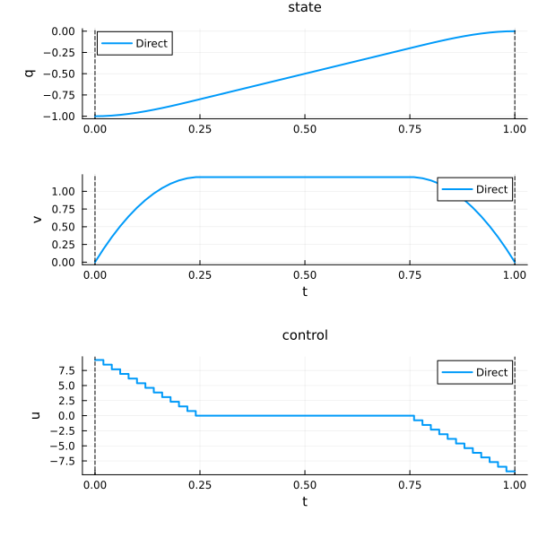

Indirect solution

The pseudo-Hamiltonian is      . Off the boundary,  ; on it,   and the multiplier is   (see Constrained arcs for this construction in general — same problem, same constraint):

f_interior = Flow(ocp, (x, p) -> p[2])

g(x) = VMAX - x[2]
μ(x, p) = p[1]

f_boundary = Flow(ocp, (x, p) -> 0.0; constraint=:vmax, multiplier=μ)

OptimalControlFlow
├─ system: HamiltonianSystem
│  ├─ time_dependence: Autonomous
│  ├─ variable_dependence: Fixed
│  ├─ ComposedHamiltonian: autonomous, fixed (no variable)
│  │    natural call: h(x, p)
│  │    uniform call: h(t, x, p, v)
│  └─ backend: DifferentiationInterface{CPU}(ad_backend=AutoForwardDiff)
└─ integrator: SciML{CPU} (instance, id=:sciml)
   ├─ internalnorm = real_norm  [default]
   ├─ alg = Tsit5  [default]
   ├─ reltol = 1.0e-8  [default]
   ├─ save_everystep = auto  [default]
   ├─ abstol = 1.0e-8  [default]
   ├─ save_start = auto  [default]
   └─ dense = auto  [default]
   Tip: use describe(SciML{CPU}) to see all available options.

Three arcs — unconstrained, boundary, unconstrained — joined at the entry time and exit time :

function shoot!(s, ξ)
    p0, t1, t2 = ξ[1:2], ξ[3], ξ[4]

    x_t1, p_t1 = f_interior(t0, x0, p0, t1)
    x_t2, p_t2 = f_boundary(t1, x_t1, p_t1, t2)
    x_tf, _ = f_interior(t2, x_t2, p_t2, tf)

    s[1:2] = x_tf - xf
    s[3] = g(x_t1)     # entry: v(t1) = VMAX
    s[4] = p_t1[2]     # switching condition
    return nothing
end

shoot! (generic function with 1 method)

nle!(s, ξ, _) = shoot!(s, ξ)

t_grid = time_grid(direct_sol)
x_of_t = state(direct_sol)
p_of_t = costate(direct_sol)

p0_guess = p_of_t(t0)
active = findall(t -> 0 ≤ g(x_of_t(t)) ≤ 1e-2, t_grid)
t1_guess = t_grid[first(active)]
t2_guess = t_grid[last(active)]

ξ_guess = [p0_guess..., t1_guess, t2_guess]

prob = NonlinearProblem(nle!, ξ_guess)
shooting_sol = NonlinearSolve.solve(prob; show_trace=Val(false))
p0_sol, t1_sol, t2_sol = shooting_sol.u[1:2], shooting_sol.u[3], shooting_sol.u[4]

([8.357548079234304, 4.478628739933972], 0.5358783099389736, 0.686654416976805)

s = zeros(4)
shoot!(s, shooting_sol.u)
s

4-element Vector{Float64}:
 -2.1187411044016544e-14
 -2.0214869084983184e-14
 -1.9095836023552692e-14
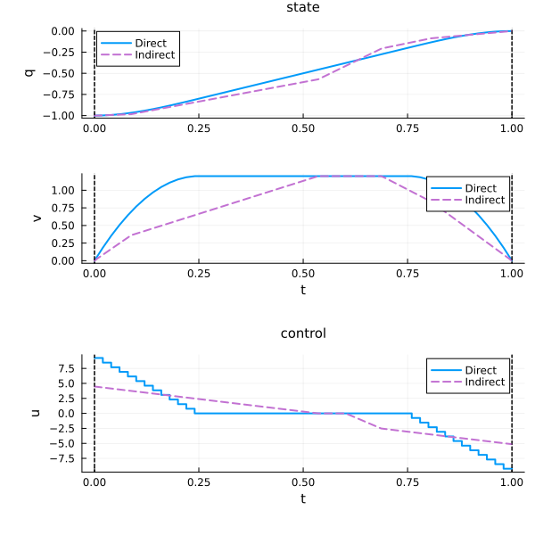
  1.808259726101572e-13

Comparison

φ = f_interior * (t1_sol, f_boundary) * (t2_sol, f_interior)
indirect_sol = φ((t0, tf), x0, p0_sol)
plot!(plt, indirect_sol, :state, :control; label="Indirect", linestyle=:dash)

Second-order constraint: bounding the position

The problem

A different pair of boundary conditions,  ,   , constraining the position   instead of the velocity. Since doesn't appear in , this is a second-order state constraint — the boundary arc forces   (not   directly), and the costate picks up a jump, not a nonzero running multiplier.

t0b = 0.0
tfb = 1.0
x0_bd = [0.0, 1.0]
xf_bd = [0.0, -1.0]

function make_ocp(a)
    @def begin
        t ∈ [t0b, tfb], time
        x = (q, v) ∈ R², state
        u ∈ R, control

        x(t0b) == x0_bd
        x(tfb) == xf_bd

        q(t) ≤ a

        ẋ(t) == [v(t), u(t)]

        0.5∫(u(t)^2) → min
    end
end

Two regimes, depending on how tight is: a touch point (the trajectory grazes   at a single instant) for a loose bound, and a genuine boundary arc for a tight one.

Touch-point case ( )

a_touch = 0.2
ocp_touch = make_ocp(a_touch)
sol_touch = solve(ocp_touch; grid_size=100, display=false)

fs_touch = Flow(ocp_touch, (x, p) -> p[2])
g_touch(x) = a_touch - x[1]

g_touch (generic function with 1 method)

Two unconstrained arcs meeting at the contact instant , where  ,  , and the costate's -component jumps by :

function shoot_touch!(s, ξ)
    p0, t1, Δpq = ξ[1:2], ξ[3], ξ[4]

    x_t1, p_t1 = fs_touch(t0b, x0_bd, p0, t1)
    p_t1_plus = [p_t1[1] + Δpq, p_t1[2]]
    x_tf, _ = fs_touch(t1, x_t1, p_t1_plus, tfb)

    s[1:2] = x_tf - xf_bd
    s[3] = g_touch(x_t1)
    s[4] = x_t1[2]
    return nothing
end

shoot_touch! (generic function with 1 method)

nle_touch!(s, ξ, _) = shoot_touch!(s, ξ)

t_grid_t = time_grid(sol_touch)
p_of_t_touch = costate(sol_touch)

p0_guess_t = p_of_t_touch(t0b)
t1_guess_t = t_grid_t[argmin(abs.(g_touch.(state(sol_touch).(t_grid_t))))]
ε = 0.05 * (tfb - t0b)
Δpq_guess = p_of_t_touch(t1_guess_t + ε)[1] - p_of_t_touch(t1_guess_t - ε)[1]

prob_touch = NonlinearProblem(nle_touch!, [p0_guess_t..., t1_guess_t, Δpq_guess])
shoot_sol_touch = NonlinearSolve.solve(prob_touch; show_trace=Val(false))
p0_touch, t1_touch, Δpq_touch = shoot_sol_touch.u[1:2], shoot_sol_touch.u[3], shoot_sol_touch.u[4]

([-4.800000000000061, -3.200000000000015], 0.49999999999999784, 9.600000000000042)

f_touch = fs_touch * (t1_touch, [Δpq_touch, 0.0], fs_touch)
indirect_touch = f_touch((t0b, tfb), x0_bd, p0_touch)
plt2 = plot(indirect_touch, :state, :control; label="Indirect (a = 0.2)")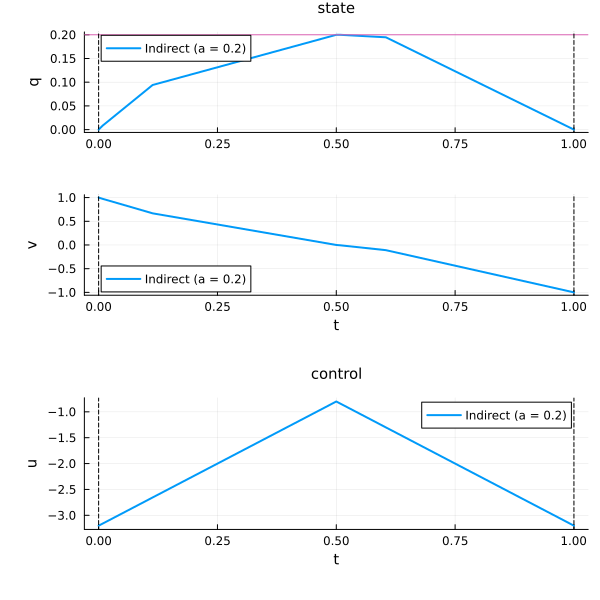

Boundary-arc case ( )

A tighter bound turns the touch point into a genuine third arc, , on which  ,  ,   — and the costate jumps twice, once on entry and once on exit:

a_arc = 0.1
ocp_arc = make_ocp(a_arc)
sol_arc = solve(ocp_arc; grid_size=100, display=false)

fs_arc = Flow(ocp_arc, (x, p) -> p[2])
g_arc(x) = a_arc - x[1]

fc_bd = Flow(ocp_arc, (x, p) -> 0.0; constraint=(x, u) -> g_arc(x), multiplier=(x, p) -> 0.0)

OptimalControlFlow
├─ system: HamiltonianSystem
│  ├─ time_dependence: Autonomous
│  ├─ variable_dependence: Fixed
│  ├─ ComposedHamiltonian: autonomous, fixed (no variable)
│  │    natural call: h(x, p)
│  │    uniform call: h(t, x, p, v)
│  └─ backend: DifferentiationInterface{CPU}(ad_backend=AutoForwardDiff)
└─ integrator: SciML{CPU} (instance, id=:sciml)
   ├─ internalnorm = real_norm  [default]
   ├─ alg = Tsit5  [default]
   ├─ reltol = 1.0e-8  [default]
   ├─ save_everystep = auto  [default]
   ├─ abstol = 1.0e-8  [default]
   ├─ save_start = auto  [default]
   └─ dense = auto  [default]
   Tip: use describe(SciML{CPU}) to see all available options.

function shoot_arc!(s, ξ)
    p0, t1, t2, Δpq1, Δpq2 = ξ[1:2], ξ[3], ξ[4], ξ[5], ξ[6]

    x_t1, p_t1 = fs_arc(t0b, x0_bd, p0, t1)
    p_t1_plus = [p_t1[1] + Δpq1, p_t1[2]]
    x_t2, p_t2 = fc_bd(t1, x_t1, p_t1_plus, t2)
    p_t2_plus = [p_t2[1] + Δpq2, p_t2[2]]
    x_tf, _ = fs_arc(t2, x_t2, p_t2_plus, tfb)

    s[1:2] = x_tf - xf_bd
    s[3] = g_arc(x_t1)
    s[4] = x_t1[2]
    s[5] = p_t1_plus[2]
    s[6] = p_t1_plus[1]
    return nothing
end

shoot_arc! (generic function with 1 method)

nle_arc!(s, ξ, _) = shoot_arc!(s, ξ)

t_grid_a = time_grid(sol_arc)
x_of_t_a = state(sol_arc)
p_of_t_a = costate(sol_arc)

p0_guess_a = p_of_t_a(t0b)
active_a = findall(t -> 0 ≤ g_arc(x_of_t_a(t)) ≤ 1e-2, t_grid_a)
t1_guess_a = t_grid_a[first(active_a)]
t2_guess_a = t_grid_a[last(active_a)]

εa = 0.1 * (tfb - t0b)
Δpq1_guess = p_of_t_a(t1_guess_a + εa)[1] - p_of_t_a(t1_guess_a - εa)[1]
Δpq2_guess = p_of_t_a(t2_guess_a + εa)[1] - p_of_t_a(t2_guess_a - εa)[1]

ξ_guess_a = [p0_guess_a..., t1_guess_a, t2_guess_a, Δpq1_guess, Δpq2_guess]

prob_arc = NonlinearProblem(nle_arc!, ξ_guess_a)
shoot_sol_arc = NonlinearSolve.solve(prob_arc; show_trace=Val(false))
p0_arc = shoot_sol_arc.u[1:2]
t1_arc, t2_arc = shoot_sol_arc.u[3], shoot_sol_arc.u[4]
Δpq1, Δpq2 = shoot_sol_arc.u[5], shoot_sol_arc.u[6]

(22.222222222222758, 22.22222222222199)

s = zeros(6)
shoot_arc!(s, shoot_sol_arc.u)
s

6-element Vector{Float64}:
 -9.943102150357695e-16
 -1.1102230246251565e-15
 -1.249000902703301e-16
 -7.920259483838119e-16
 -1.5708663185183915e-15
  0.0

f_arc = fs_arc * (t1_arc, [Δpq1, 0.0], fc_bd) * (t2_arc, [Δpq2, 0.0], fs_arc)
indirect_arc = f_arc((t0b, tfb), x0_bd, p0_arc)
plot!(plt2, indirect_arc, :state, :control; label="Indirect (a = 0.1)")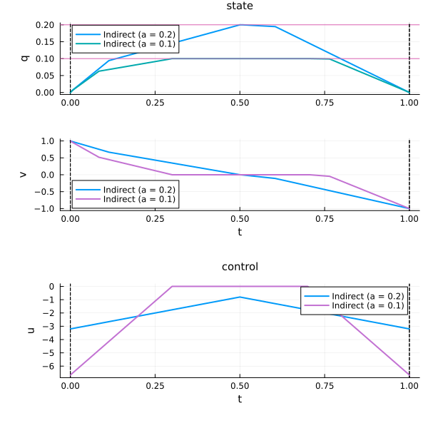

By symmetry of the problem, the entry and exit times should be close to and  :

t1_arc, 3a_arc, t2_arc, 1 - 3a_arc

(0.29999999999999594, 0.30000000000000004, 0.6999999999999981, 0.7)

See also

• Constrained arcs — constraint=/multiplier=, the three ways to spell the constraint, in general.

• Multi-phase — flow concatenation and costate jumps, in general.

• Energy minimisation — the same wagon, unconstrained.