Plot

plot/plot! extend Plots.jl to draw a Solution directly — the same call works on a Flow-produced trajectory too (last section below). The full signatures are collected under Reference at the end.

Choosing a backend. Plots is the default and what this page documents. A second backend, Makie.jl, draws the same figures at feature parity — worth it for an interactive window, or if you already draw in Makie elsewhere. See Plot with Makie.

Getting started

using OptimalControl
using NLPModelsIpopt

t0 = 0
tf = 1
x0 = [-1, 0]
xf = [0, 0]

ocp = @def begin
    t ∈ [t0, tf], time
    x ∈ R², state
    u ∈ R, control
    x(t0) == x0
    x(tf) == xf
    ẋ(t) == [x₂(t), u(t)]
    ∫(0.5u(t)^2) → min
end

sol = solve(ocp; display=false)

plot on a solution is an extension — nothing is drawn until Plots itself is loaded:

using Plots
plot(sol)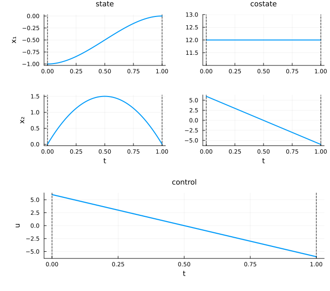

Without Plots in the session the call throws a clean ExtensionError instead:

julia> using OptimalControl
julia> plot(sol)
ERROR: ExtensionError: missing dependencies to plot solutions
Missing  Plots
Hint     Run: using Plots

What gets drawn by default

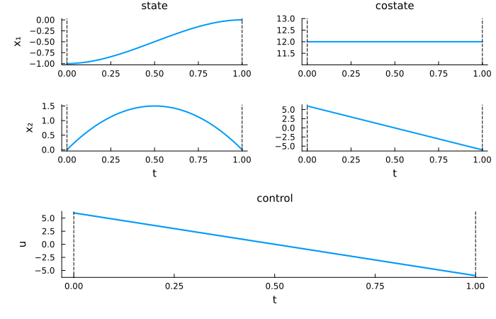
With every group shown, the layout is a grid: state trajectories on the left, costate on the right, control along the bottom.

plot(
    sol, :state, :costate, :control;
    size=(700, 450), legend=:bottomright, grid=false, linewidth=2,
)

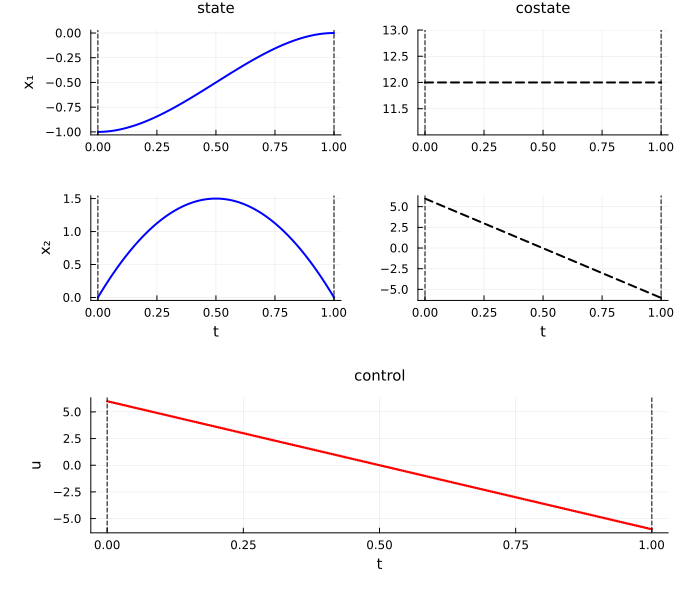
state_style, costate_style, and control_style set series attributes per group (any Plots.jl attribute, as a NamedTuple):

plot(sol, :state, :costate, :control;
    state_style=(color=:blue,),
    costate_style=(color=:black, linestyle=:dash),
    control_style=(color=:red, linewidth=2),
)

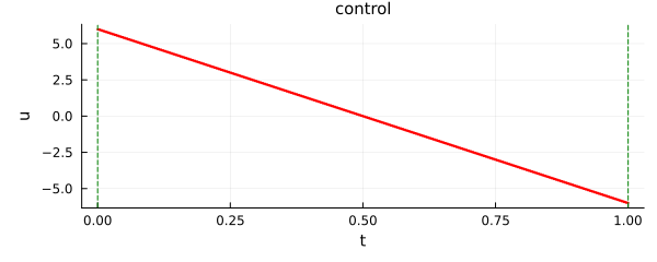
Vertical markers at the initial/final times are controlled by time_style. Any *_style also accepts :none to hide that group entirely:

plot(sol, :state, :costate, :control;
    state_style=:none,
    costate_style=:none,
    control_style=(color=:red,),
    time_style=(color=:green,),
)

Choosing what to draw

Positional symbols select which groups appear — :state, :costate, :control, and (with a path constraint present) :path, :dual:

plot(sol, :state)    # only the state
plot(sol, :costate)  # only the costate
plot(sol, :control)  # only the control

Combine freely:

plot(sol, :state, :control)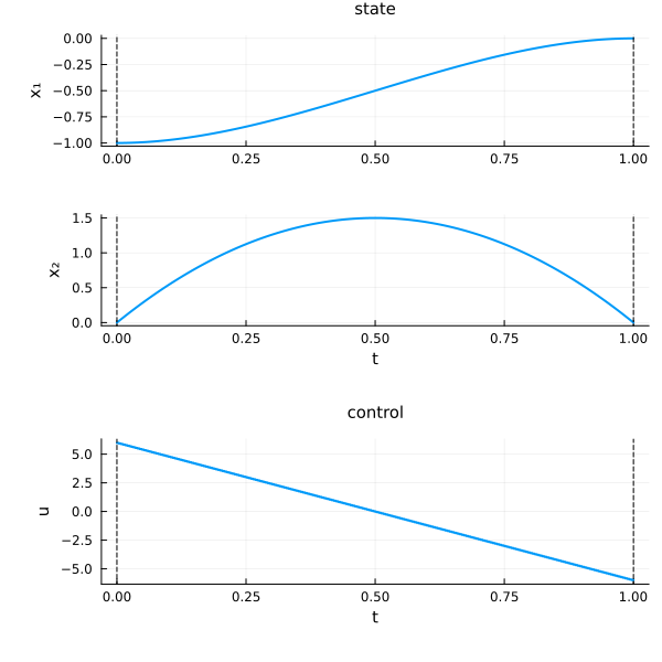

Layout

layout=:group puts each family (state, costate, control) in one subplot instead of one per component:

plot(sol; layout=:group)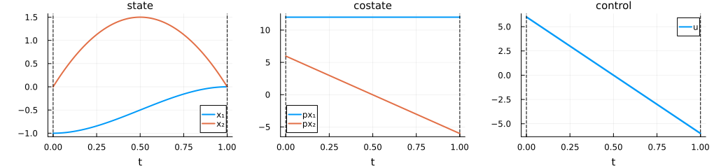

:split (the default) is the per-component grid used everywhere above.

The control

control=:norm plots the Euclidean norm of the control instead of its components; control=:all plots both:

plot(sol; control=:norm, layout=:group, size=(800, 300))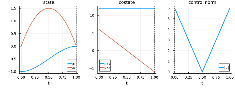

plot(sol; control=:components, layout=:group, size=(800, 300))  # default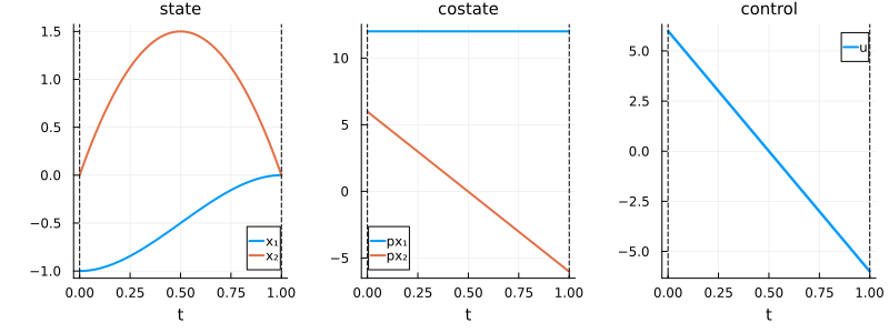

plot(sol; control=:all, layout=:group)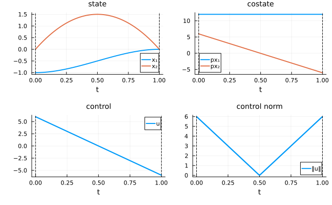

Styling

Covered above (state_style/costate_style/control_style/time_style) — repeated here for the outline: every one of them is a NamedTuple of Plots.jl attributes, or :none to hide the group. Use plotattr("attribute") (from Plots) to look up any attribute's aliases and description once using Plots is loaded.

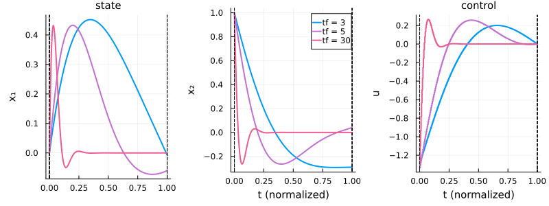
Normalised time

Solve the same problem for several final times and compare them on a normalised time axis    , via time=:normalize (or the British spelling, :normalise — both work):

function lqr(tf)
    ocp = @def begin
        t ∈ [0, tf], time
        x ∈ R², state
        u ∈ R, control
        x(0) == [0, 1]
        ẋ(t) == [x₂(t), -x₁(t) + u(t)]
        ∫(0.5(x₁(t)^2 + x₂(t)^2 + u(t)^2)) → min
    end
    return ocp
end

tfs = [3, 5, 30]
solutions = [solve(lqr(tf); display=false) for tf in tfs]

plt = plot()
for (tf, sol) in zip(tfs, solutions)
    plot!(
        plt, sol, :state, :control;
        time=:normalize, label="tf = $tf", xlabel="s",
    )
end

using Plots.PlotMeasures
px1 = plot(plt[1]; legend=false)  # x₁
px2 = plot(plt[2]; legend=true)   # x₂
pu = plot(plt[3]; legend=false)   # u
plot(
    px1, px2, pu;
    layout=(1, 3), size=(800, 300), leftmargin=5mm, bottommargin=5mm,
)

Constraints

A problem with a box control constraint and a nonlinear path constraint:

ocp_c = @def begin
    tf ∈ R, variable
    t ∈ [0, tf], time
    x = (q, v) ∈ R², state
    u ∈ R, control
    tf ≥ 0
    -1 ≤ u(t) ≤ 1
    q(0) == -1
    v(0) == 0
    q(tf) == 0
    v(tf) == 0
    1 ≤ v(t) + 1 ≤ 1.8, (c1)
    ẋ(t) == [v(t), u(t)]
    tf → min
end
sol_c = solve(ocp_c; display=false)
plot(sol_c, :state, :costate, :control, :path, :dual)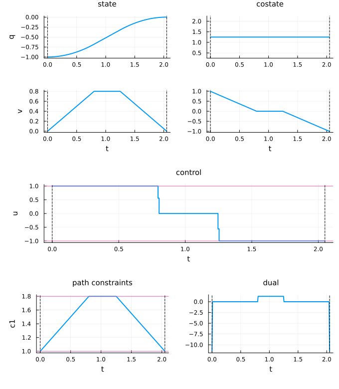

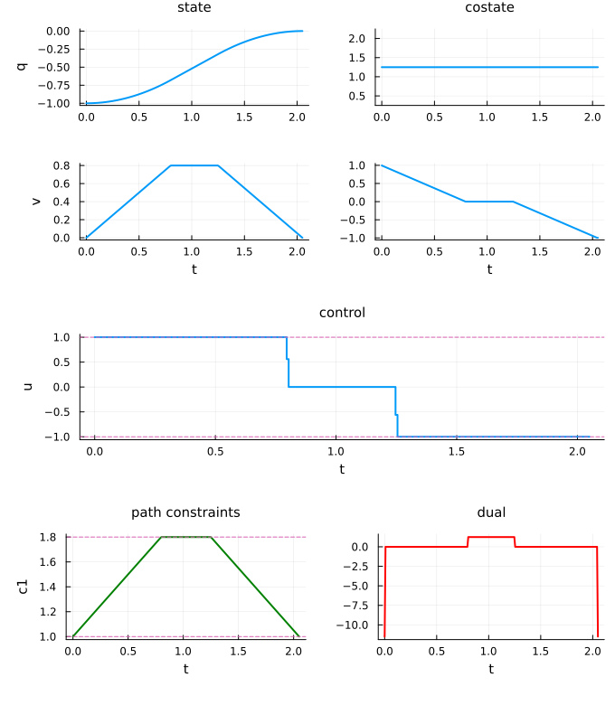
The path constraint's bounds are drawn alongside it, with its dual variable in its own panel. Style keywords for these two extra groups: path_style, dual_style, and the bounds decorations state_bounds_style, control_bounds_style, path_bounds_style:

plot(sol_c, :state, :costate, :control, :path, :dual;
    state_bounds_style=(linestyle=:dash,),
    control_bounds_style=(linestyle=:dash,),
    path_style=(color=:green,),
    path_bounds_style=(linestyle=:dash,),
    dual_style=(color=:red,),
    time_style=:none,
)

Adding to an existing plot

plot! overlays a second solution — same state/costate/control dimensions required:

ocp2 = @def begin
    t ∈ [t0, tf], time
    x ∈ R², state
    u ∈ R, control
    x(t0) == [-0.5, -0.5]
    x(tf) == xf
    ẋ(t) == [x₂(t), u(t)]
    ∫(0.5u(t)^2) → min
end
sol2 = solve(ocp2; display=false)

plt = plot(sol, :state, :costate, :control; label="sol1", size=(700, 500))
plot!(plt, sol2, :state, :costate, :control; label="sol2", linestyle=:dash)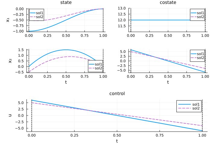

Custom subplots

Extract state, control, costate as plain functions to build your own figure:

using LinearAlgebra
t = time_grid(sol)
u = control(sol)
plot(t, norm ∘ u; label="‖u‖", xlabel="t")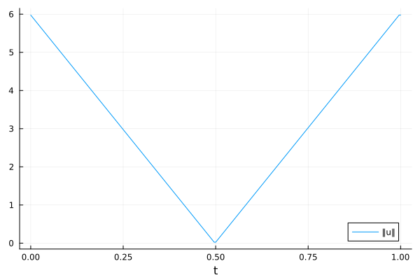

Or reach into an existing plot(sol, ...)'s subplots directly — order follows the :state, :costate, :control, :path, :dual grouping, in the order requested:

plt = plot(sol, :state, :costate, :control)
plot(plt[1])  # x₁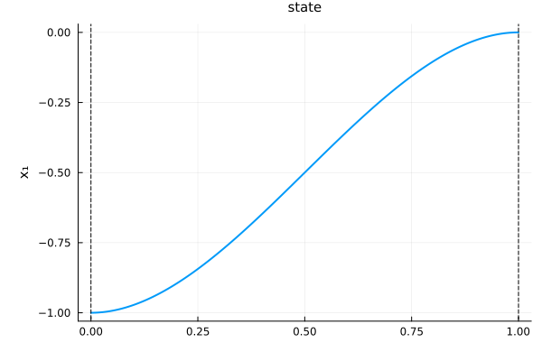

plot(plt[5])  # u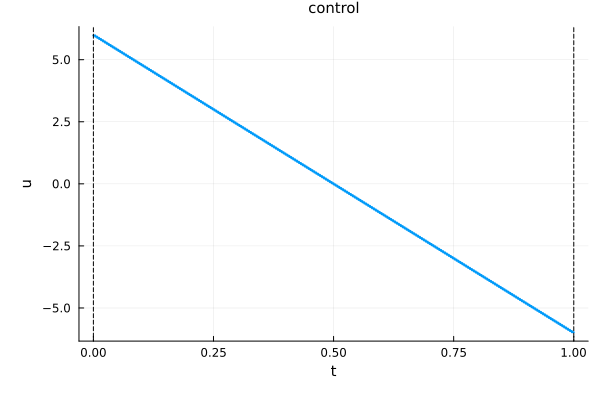

A subplot also accepts native Plots calls directly, to annotate rather than re-plot it — for example marking a control bound:

plot(plt[5])
hline!([-1, 1]; linestyle=:dash, color=:red)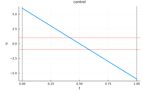

The same idea, in Makie, needs one extra step — a panel there is an Axis, not a subplot — see Plot with Makie.

Plotting a flow trajectory

The same plot call works on a trajectory produced by Flow — see Flows for how to build one; here's the plotting side:

using OrdinaryDiffEqTsit5

p = costate(sol)
p0 = p(t0)
f = Flow(ocp, (x, p) -> p[2])  # flow from an ocp + a feedback law

sol_flow = f((t0, tf), x0, p0)
plot(sol_flow)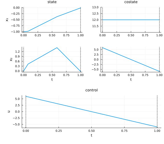

The default grid can be sparse — the subplot above shows it, or read it directly:

time_grid(sol_flow)

5-element Vector{Float64}:
 0.0
 0.00694633729453733
 0.07787622341383321
 0.5858181009164434
 1.0

For a denser plot, pass saveat when constructing the flow, not on the call — the call itself only accepts variable/unsafe (and variable_costate, for costate augmentation). dense=false is required alongside saveat, since dense output and saveat conflict at the integrator level:

fine_grid = range(t0, tf, 100)
f2 = Flow(ocp, (x, p) -> p[2]; saveat=fine_grid, dense=false)
sol_flow2 = f2((t0, tf), x0, p0)
plot(sol_flow2)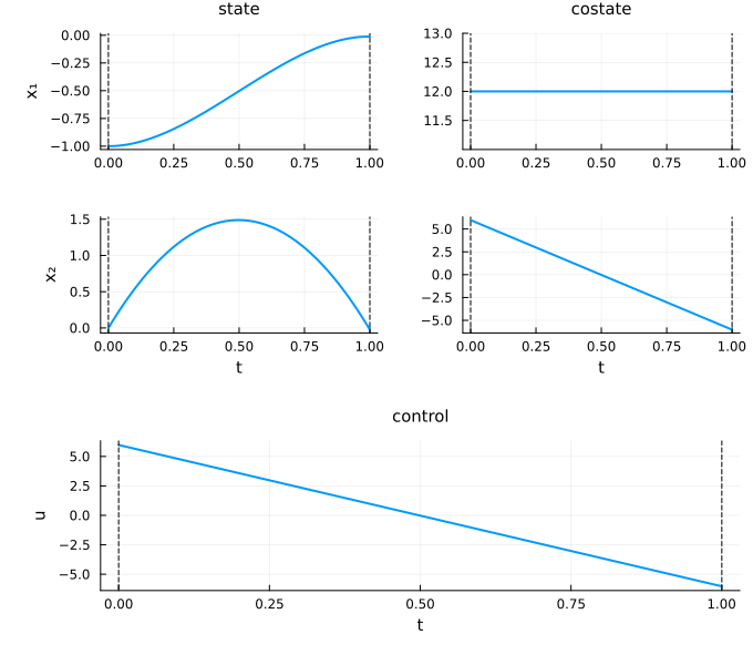

Reference

RecipesBase.plot Method

plot(
    sol::CTModels.Solutions.Solution,
    description::Symbol...;
    kwargs...
) -> Any

Plot the components of an optimal control CTModels.Solutions.Solution.

Generates a set of subplots showing the state, control, costate, path constraints and dual variables over time, depending on the problem and the given description.

Arguments

• sol: the optimal control solution to visualise.

• description: symbols selecting which groups to include; any of :state, :costate, :control, :path (path constraints), :dual (their multipliers). If none is given, a default set is used based on the problem.

Keyword arguments

• layout::Symbol = :split: :split (one subplot per component) or :group (group each signal into a single subplot with a legend).

• control::Symbol = :components: :components (a curve per control component), :norm (the Euclidean norm ‖u(t)‖) or :all (both).

• time::Symbol = :default: :default (real time) or :normalize/:normalise ([0, 1]).

• color: colour applied to every curve.

• size: figure size; defaults to a heuristic based on the layout.

Style options

Each *_style keyword is a NamedTuple of plotting attributes, or :none to hide the group/decoration: state_style, costate_style, control_style, path_style, dual_style, time_style (initial/final time markers), and the bounds decorations state_bounds_style, control_bounds_style, path_bounds_style.

Returns

A Plots.Plot. All layout and rendering is delegated to CTBase.Plotting.

Example

julia> plot(sol)
julia> plot(sol, :state, :control; layout=:group, control=:all)
julia> plot(sol; state_style=(color=:blue,), costate_style=:none)

RecipesBase.plot! Method

plot!(
    sol::CTModels.Solutions.Solution,
    description::Symbol...;
    kwargs...
) -> Plots.Plot

Overlay the optimal control solution sol onto the current plot (Plots.current()).

RecipesBase.plot! Method

plot!(
    p::Plots.Plot,
    sol::CTModels.Solutions.Solution,
    description::Symbol...;
    kwargs...
) -> Plots.Plot

Overlay the optimal control solution sol onto the existing plot p. Same behaviour and keyword arguments as plot (documented above); an empty p is filled as if by plot.

See also

• Solution object — the accessors this page draws.

• Save and load — persist a solution instead of just plotting it.

• Flows — building the Flow used in the last section.