
Energy minimisation
The double integrator — a unit mass sliding frictionlessly on a rail, acceleration as the control — transferred between two rest states at minimal energy. The simplest problem on this site, and the same one used to introduce the package on the home page.
using OptimalControl
using NLPModelsIpopt
using OrdinaryDiffEqTsit5
using NonlinearSolve
using Plots
The problem
State
Definition
Character-identical to the problem on the home page — this is the same instance, so the two should recognisably be the same problem:
ocp = @def begin
    t ∈ [0, 1], time
    x ∈ R², state
    u ∈ R, control
    x(0) == [-1, 0]
    x(1) == [0, 0]
    ẋ(t) == [x₂(t), u(t)]
    ∫( 0.5u(t)^2 ) → min
end
Abstract definition:
t ∈ [0, 1], time
x ∈ R², state
u ∈ R, control
x(0) == [-1, 0]
x(1) == [0, 0]
ẋ(t) == [x₂(t), u(t)]
∫(0.5 * u(t) ^ 2) → min
The (autonomous) optimal control problem is of the form:
minimize J(x, u) = ∫ f⁰(x(t), u(t)) dt, over [0, 1]
subject to
ẋ(t) = f(x(t), u(t)), t in [0, 1] a.e.,
ϕ₋ ≤ ϕ(x(0), x(1)) ≤ ϕ₊,
where x(t) ∈ R² and u(t) ∈ R.t0, tf = 0, 1
x0, xf = [-1, 0], [0, 0]Direct solution
direct_sol = solve(ocp; grid_size=20, display=false)
plt = plot(direct_sol, :state, :control; label="Direct")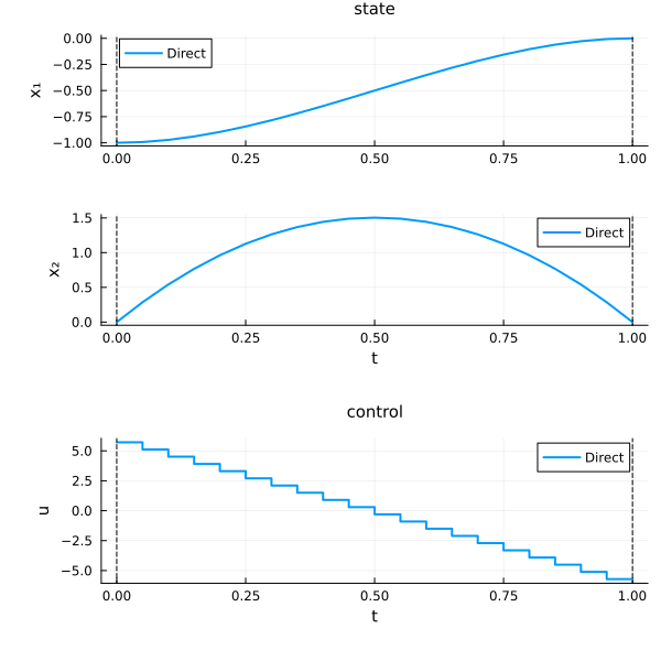
Indirect solution
The pseudo-Hamiltonian is
u(x, p) = p[2]
f = Flow(ocp, u; saveat=range(t0, tf, 100), dense=false)
OptimalControlFlow
├─ system: HamiltonianSystem
│ ├─ time_dependence: Autonomous
│ ├─ variable_dependence: Fixed
│ ├─ ComposedHamiltonian: autonomous, fixed (no variable)
│ │ natural call: h(x, p)
│ │ uniform call: h(t, x, p, v)
│ └─ backend: DifferentiationInterface{CPU}(ad_backend=AutoForwardDiff)
└─ integrator: SciML{CPU} (instance, id=:sciml)
├─ internalnorm = real_norm [default]
├─ alg = Tsit5 [default]
├─ reltol = 1.0e-8 [default]
├─ save_everystep = auto [default]
├─ saveat = 0.0:0.010101010101010102:1.0 [user]
├─ abstol = 1.0e-8 [default]
├─ save_start = auto [default]
└─ dense = false [user]
Tip: use describe(SciML{CPU}) to see all available options.The shooting function drives the flow's endpoint to the target:
π_x((x, p)) = x
S(p0) = π_x(f(t0, x0, p0, tf)) - xf
S (generic function with 1 method)nle!(s, p0, _) = (s .= S(p0))
t = time_grid(direct_sol)
p0_guess = costate(direct_sol)(t0)
prob = NonlinearProblem(nle!, p0_guess)
shooting_sol = NonlinearSolve.solve(prob; show_trace=Val(false))
p0_sol = shooting_sol.u2-element Vector{Float64}:
12.000000000000062
6.000000000000017S(p0_sol)2-element Vector{Float64}:
3.1827698819287482e-15
1.4077143355866606e-14Comparison
indirect_sol = f((t0, tf), x0, p0_sol)
plot!(plt, indirect_sol, :state, :control; label="Indirect")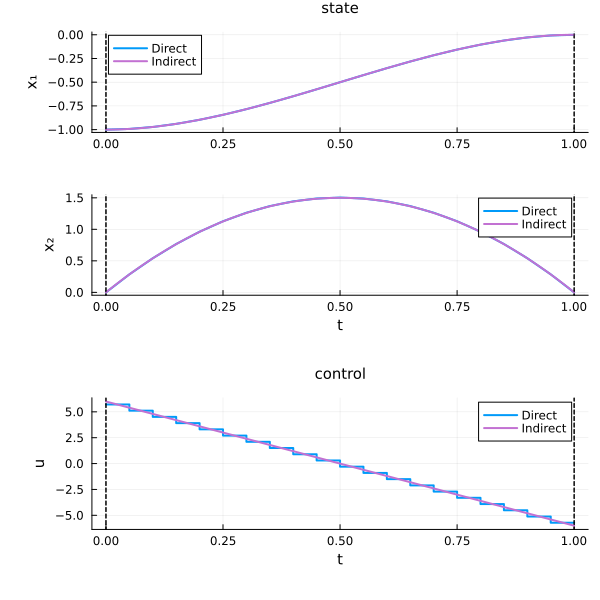
The two solutions overlap: the shooting function's residual at p0_sol is numerically zero, confirming the indirect solve reproduces the direct one.
See also
From an OCP — the Hamiltonian-flow construction used above, in full.
Shooting — the shooting method in general.
Time minimisation (bang–bang) — the same wagon, a harder control constraint.