No control

What this is for

Control-free problems are optimal control problems without a control variable — used for optimising constant parameters in dynamical systems, such as:

• identifying unknown parameters from observed data (parameter estimation),

• finding optimal parameters for a given performance criterion.

This page demonstrates two examples with known analytical solutions, solved both directly and indirectly.

How to declare it

There is no dedicated syntax for "no control": simply never declare one. Declare a variable, a time, a state, dynamics, and a cost, and omit the control line entirely (on the abstract syntax) or never call control! (on the functional API).

control!(pre, 0) is an error, not a spelling for "no control"

A control-free problem is reached purely by omission. control!(pre, 0) throws IncorrectArgument — a dimension must be positive. Internally, a PreModel that never called control! keeps its default EmptyControlModel, and is_control_free/has_control read that from the type of the built model's control field, not from a dimension check.

using OptimalControl
using NLPModelsIpopt
using Plots

Worked example: exponential growth

Consider a system with exponential growth:

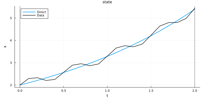
where is an unknown growth rate parameter. We have observed data with some perturbations and want to estimate by minimising the squared error:

The underlying model has  , but the observed data includes perturbations.

# observed data (analytical solution with λ = 0.5)
λ_true = 0.5
model(t) = 2 * exp(λ_true * t)
perturbation(t) = 2e-1*sin(4π*t)
data(t) = model(t) + perturbation(t)

# optimal control problem (parameter estimation)
t0 = 0; tf = 2; x0 = 2
ocp = @def begin
    λ ∈ R, variable              # growth rate to estimate
    t ∈ [t0, tf], time
    x ∈ R, state

    x(t0) == x0
    ẋ(t) == λ * x(t)

    ∫((x(t) - data(t))^2) → min  # fit to observed data
end

Direct method

direct_sol = solve(ocp; grid_size=20, display=false)

Solution  ✓ successful
  │  Objective : 0.039296407666384314
  │  λ : 0.4960778956661449
  │  Boundary duals : [0.061507876561442874]
  │
  │  Iterations : 14
  │  Status : first_order
  │  Message : Ipopt/generic
  └─ Constraints violation : 9.325873406851315e-15

println("Estimated growth rate: λ = ", variable(direct_sol))
println("Objective value: ", objective(direct_sol))

Estimated growth rate: λ = 0.4960778956661449
Objective value: 0.039296407666384314

plt = plot(direct_sol, :state; size=(800, 400), label="Direct")
t_grid = time_grid(direct_sol)
plot!(plt, t_grid, data.(t_grid); subplot=1, line=:dot, lw=2, label="Data", color=:black)

The estimated parameter should be close to  .

Indirect method

We now solve the same problem using an indirect shooting method based on Pontryagin's Maximum Principle.

using OrdinaryDiffEq  # ODE solver
using NonlinearSolve  # Nonlinear solver

For control-free problems with a variable parameter, we use an augmented Hamiltonian approach. The Hamiltonian for this problem is:

To handle the variable parameter , we treat it as an additional state with zero dynamics. This gives us the augmented system with state and costate , where:

The transversality condition for the variable parameter requires   . Assuming  , we have to satisfy:

We use variable_costate=true to automatically compute without manually constructing the augmented system.

# Create Hamiltonian flow from the control-free OCP
f = Flow(ocp)

Note

For more on building flows from an OCP, see Flows overview and From an OCP.

The shooting function enforces the transversality conditions   and  . With variable_costate=true, the flow returns , with   by construction. The variable is passed as a keyword, variable=λ:

# Shooting function: S(p0, λ) = (p(tf), pλ(tf))
function shoot!(s, p0, λ)
    _, px_tf, pλ_tf = f(t0, x0, p0, tf; variable=λ, variable_costate=true)
    s[1] = px_tf
    s[2] = pλ_tf
    return nothing
end

# Auxiliary in-place NLE function
nle!(s, y, _) = shoot!(s, y...)

We use the direct solution to initialise the shooting method:

p_direct = costate(direct_sol)
λ_direct = variable(direct_sol)

p0_guess = p_direct(t0)
λ_guess = λ_direct

prob_indirect = NonlinearProblem(nle!, [p0_guess, λ_guess])
shooting_sol = solve(prob_indirect; show_trace=Val(false))
p0_sol, λ_sol = shooting_sol.u

println("Indirect solution:")
println("Initial costate: p0 = ", p0_sol)
println("Parameter: λ = ", λ_sol)

Indirect solution:
Initial costate: p0 = 0.05847851053035069
Parameter: λ = 0.49662126696284686

Finally, we compute and plot the indirect solution — the trajectory call takes no saveat, it returns a full solution over the flow's own grid:

indirect_sol = f((t0, tf), x0, p0_sol; variable=λ_sol)
plot!(plt, indirect_sol, :state; linestyle=:dash, lw=2, label="Indirect", color=2)

The direct and indirect solutions match closely, both fitting the perturbed observed data.

Worked example: harmonic oscillator

Consider a harmonic oscillator:

with initial conditions  ,   and final condition  . We want to find the minimal pulsation satisfying these constraints:

The analytical solution is   , giving  .

q0 = 1; v0 = 0
t0 = 0; tf = 1
ocp = @def begin
    ω ∈ R, variable              # pulsation to optimize
    t ∈ [t0, tf], time
    x = (q, v) ∈ R², state

    q(t0) == q0
    v(t0) == v0
    q(tf) == 0.0                  # final condition

    ẋ(t) == [v(t), -ω^2 * q(t)]

    ω^2 → min   # minimize pulsation
end

Direct method

direct_sol = solve(ocp; grid_size=20, display=false)

Solution  ✓ successful
  │  Objective : 2.469940014156302
  │  ω : 1.5716042803951324
  │  Boundary duals : [2.776384949033009e-10, -2.003087424961417, 3.148060771075015]
  │
  │  Iterations : 9
  │  Status : first_order
  │  Message : Ipopt/generic
  └─ Constraints violation : 1.3778783669593508e-11

println("Optimal pulsation: ω = ", variable(direct_sol))
println("Objective value: ω² = ", objective(direct_sol))
println("Expected: ω = π/2 ≈ 1.5708, ω² ≈ 2.4674")

Optimal pulsation: ω = 1.5716042803951324
Objective value: ω² = 2.469940014156302
Expected: ω = π/2 ≈ 1.5708, ω² ≈ 2.4674

plot(direct_sol, :state; size=(800, 400))

Comparison with the analytical solution

t_analytical = range(0, 1, 100)
q_analytical = cos.(π * t_analytical / 2)
v_analytical = -(π/2) * sin.(π * t_analytical / 2)

plt = plot(direct_sol, :state; size=(800, 600), label="Direct")
plot!(plt, t_analytical, q_analytical;
      label="q (analytical)", linestyle=:dash, linewidth=2, subplot=1)
plot!(plt, t_analytical, v_analytical;
      label="v (analytical)", linestyle=:dash, linewidth=2, subplot=2)

The numerical and analytical solutions should match closely.

Indirect method

For this control-free problem with a variable parameter, we again use the augmented-Hamiltonian approach. The Hamiltonian is:

Treating as an additional state with zero dynamics gives the augmented system with state and costate :

For a Mayer cost  , the transversality condition for the variable parameter is      ; assuming  :

f = Flow(ocp)

The shooting function enforces:   (final condition),   (free final velocity), and    (Mayer-cost transversality). With variable_costate=true, the flow returns , with   by construction:

function shoot!(s, p0, ω)
    x_tf, p_tf, pω_tf = f(t0, [q0, v0], p0, tf; variable=ω, variable_costate=true)
    q_tf = x_tf[1]
    pv_tf = p_tf[2]
    s[1] = q_tf         # q(tf) = 0
    s[2] = pv_tf        # p2(tf) = 0 (free final velocity)
    s[3] = pω_tf + 2ω   # pω(tf) + 2ω = 0 (Mayer cost transversality)
    return nothing
end

nle!(s, y, _) = shoot!(s, y[1:2], y[3])

p_direct = costate(direct_sol)
ω_direct = variable(direct_sol)

p0_guess = p_direct(t0)
ω_guess = ω_direct

prob_indirect = NonlinearProblem(nle!, [p0_guess..., ω_guess])
shooting_sol = solve(prob_indirect; show_trace=Val(false))
p0_sol, ω_sol = shooting_sol.u[1:2], shooting_sol.u[3]

println("Indirect solution:")
println("Initial costate: p0 = ", p0_sol)
println("Parameter: ω = ", ω_sol)

Indirect solution:
Initial costate: p0 = [7.43711190721863e-15, -2.000000000959038]
Parameter: ω = 1.570796326752619

indirect_sol = f((t0, tf), [q0, v0], p0_sol; variable=ω_sol)
plot!(plt, indirect_sol, :state; linestyle=:dash, lw=2, label="Indirect", color=2)

The direct and indirect solutions match closely, both finding the optimal pulsation  .

How the package knows

is_control_free(ocp) and has_control(ocp) don't check a dimension — they read the type of the built model's control field. A PreModel that never called control! keeps its default EmptyControlModel; build copies that straight into the immutable Model, and is_control_free dispatches on that type. There is nothing to configure: reaching ControlFree is purely a consequence of never calling control!.

Adding a control back

To turn either of these examples into a controlled problem, declare a control and give Flow a control law: Flow(ocp, law). Two guards are worth knowing before you try:

• Flow(ocp) — no law — only works on a control-free model. On a model with a control it throws PreconditionError("Flow from a with-control OCP is not supported"), suggesting Flow(ocp, law).

• constraint=/multiplier= on a control-free Flow(ocp) are rejected — PreconditionError ("constrained flows are not supported for control-free problems") — there is no control law and so no pseudo-Hamiltonian to carry a   term. Use Flow(ocp, law; constraint=…, multiplier=…) instead.

See Parameter estimation without a control for a worked example with both.

See also

• Formulation — the control-free case,  .

• Abstract syntax (@def) — the control-free syntax.

• Functional API — the control-free functional-API form.

• From an OCP — building flows in general.