Turnpike (bang–singular–bang)

A scalar system,   with   , driven between two states over a fixed horizon while minimising . Because the cost is linear in , the optimal control is bang —    — except on an interval where the switching function vanishes: a singular arc. This is the smallest problem that shows one, and unlike Singular control the singular feedback falls straight out of the optimality conditions, with no Poisson brackets.

using OptimalControl
using NLPModelsIpopt
using OrdinaryDiffEqTsit5
using NonlinearSolve
using Plots

The problem

State , control   , dynamics  , fixed horizon  , transfer from   to   minimising  . One dimension, so the state and the control are scalars, not length-1 vectors.

Definition

t0, tf = 0.0, 2.0
x0, xf = 1.0, 0.5

ocp = @def begin
    t ∈ [t0, tf], time
    x ∈ R, state
    u ∈ R, control
    -1 ≤ u(t) ≤ 1
    x(t0) == x0
    x(tf) == xf
    ẋ(t) == u(t)
    ∫(x(t)^2) → min
end

Abstract definition:

    t ∈ [t0, tf], time
    x ∈ R, state
    u ∈ R, control
    -1 ≤ u(t) ≤ 1
    x(t0) == x0
    x(tf) == xf
    ẋ(t) == u(t)
    ∫(x(t) ^ 2) → min

The (autonomous) optimal control problem is of the form:

    minimize  J(x, u) = ∫ f⁰(x(t), u(t)) dt, over [0.0, 2.0]

    subject to

        ẋ(t) = f(x(t), u(t)), t in [0.0, 2.0] a.e.,

        ϕ₋ ≤ ϕ(x(0.0), x(2.0)) ≤ ϕ₊, 
        u₋ ≤ u(t) ≤ u₊, 

    where x(t) ∈ R and u(t) ∈ R.

Direct solution

direct_sol = solve(ocp; grid_size=100, display=false)
plt = plot(direct_sol, :state, :control; label="Direct")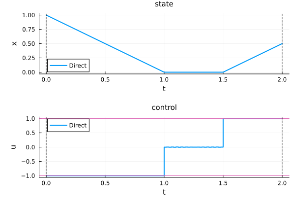

The state slides down to the origin, holds there, then climbs to the target. The flat middle stretch — the turnpike — is the singular arc, where leaves the bounds and sits at .

The singular control

The pseudo-Hamiltonian     is linear in , so the maximising control is bang,  , driven by the sign of the costate. Where vanishes on a whole interval rather than at an isolated instant, that rule says nothing and the control is singular. Differentiate  : the adjoint equation is    , so   forces  , and then   forces

The whole extremal is therefore bang–singular–bang:

arc	interval
bang down
singular
bang up

with  ,   and   , all read off by integrating each arc by hand: falls at unit rate from , reaching at  ; it rises at unit rate to , so it must leave the arc at  .

Indirect solution

Three constant-control flows, one per arc:

f_minus = Flow(ocp, (x, p) -> -1.0)
f_sing  = Flow(ocp, (x, p) ->  0.0)
f_plus  = Flow(ocp, (x, p) -> +1.0)

OptimalControlFlow
├─ system: HamiltonianSystem
│  ├─ time_dependence: Autonomous
│  ├─ variable_dependence: Fixed
│  ├─ ComposedHamiltonian: autonomous, fixed (no variable)
│  │    natural call: h(x, p)
│  │    uniform call: h(t, x, p, v)
│  └─ backend: DifferentiationInterface{CPU}(ad_backend=AutoForwardDiff)
└─ integrator: SciML{CPU} (instance, id=:sciml)
   ├─ internalnorm = real_norm  [default]
   ├─ alg = Tsit5  [default]
   ├─ reltol = 1.0e-8  [default]
   ├─ save_everystep = auto  [default]
   ├─ abstol = 1.0e-8  [default]
   ├─ save_start = auto  [default]
   └─ dense = auto  [default]
   Tip: use describe(SciML{CPU}) to see all available options.

The unknowns are the initial costate and the two switching times  ; the horizon is fixed. Three conditions close the system — the trajectory enters the singular arc at   with the switching function already vanishing there ( ), and it hits the target at :

function shoot!(s, ξ)
    p0, t1, t2 = ξ[1], ξ[2], ξ[3]
    x1, p1 = f_minus(t0, x0, p0, t1)
    x2, p2 = f_sing(t1, x1, p1, t2)
    xf_, _ = f_plus(t2, x2, p2, tf)
    s[1] = x1        # enter the singular arc at x = 0
    s[2] = p1        # switching function vanishes there
    s[3] = xf_ - xf  # hit the target
    return nothing
end

shoot! (generic function with 1 method)

For a starting point, solve the same problem directly first, then read the singular arc off that solution. The switching function here is just the costate ( ), so the arc is where stays near zero — the same recipe as the Goddard tutorial:

t = time_grid(direct_sol)
p = costate(direct_sol)

φ(τ) = p(τ)                     # switching function ≡ costate
η = 1e-3
t12 = t[abs.(φ.(t)) .≤ η]       # grid points on the singular arc

p0_guess = p(t0)
t1_guess = minimum(t12)
t2_guess = maximum(t12)
(p0_guess, t1_guess, t2_guess)

(-0.9801999456479715, 0.96, 1.52)

nle!(s, ξ, _) = shoot!(s, ξ)
prob = NonlinearProblem(nle!, [p0_guess, t1_guess, t2_guess])
shooting_sol = NonlinearSolve.solve(prob; show_trace=Val(false))
p0_sol, t1_sol, t2_sol = shooting_sol.u

3-element Vector{Float64}:
 -1.0000000000000036
  1.0000000000000002
  1.4999999999999998

s = zeros(3)
shoot!(s, shooting_sol.u)
s

3-element Vector{Float64}:
 8.034495536742733e-17
 4.696458266519542e-16
 1.1102230246251565e-16

The solver lands on   ,  ,   — the hand computation above.

Comparison

Concatenating the three constant-control flows at the solved switching times rebuilds the whole trajectory:

φ_bsb = f_minus * (t1_sol, f_sing) * (t2_sol, f_plus)
indirect_sol = φ_bsb((t0, tf), x0, p0_sol)
plot!(plt, indirect_sol, :state, :control;
    label="Indirect", linestyle=:dash)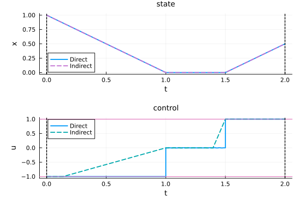

The two curves overlap, and the objective is the expected :

objective(direct_sol)

0.3749500107307793

See also

• Singular control — a 2-D drift system where the singular control does need the Lift/@Lie Poisson-bracket chain.

• Shooting — the shooting method in general; this page is a worked case of switching times as unknowns.

• Time minimisation (bang–bang) — the bang arcs on their own, with no singular arc between them.

• Multi-phase flows — concatenating arc flows with *.

• Goddard problem — the same direct-then-indirect workflow on a harder instance: a singular arc and a state-constraint boundary arc.