Functional API

The @def macro provides a concise DSL to define optimal control problems. An alternative is the functional API, which builds the same problem step by step using plain Julia functions.

The functional API uses OptimalControl.PreModel as a mutable builder, populated by setter calls, then frozen into an immutable OptimalControl.Model by build. Both PreModel and Model are imported, not exported — write OptimalControl.PreModel().

Note

When a problem is defined with the functional API, definition(ocp) returns an EmptyDefinition — no abstract expression is stored. This contrasts with @def, which records the full DSL expression for display and introspection.

Modeler compatibility

Problems built with the functional API can only be solved with the :adnlp modeler (the default). The :exa modeler (ExaModels, GPU-capable) requires the abstract syntax @def. See Solve overview for modeler details.

When you want this

• generating problems programmatically from parameters, data, or loops,

• building library code that must not rely on macros,

• interfacing with external tools that process problem structures directly.

The canvas

The functional API mirrors the Formulation. The correspondence is:

Math	Functional API
Dynamics	dyn! passed to dynamics!
Lagrange integrand	lag passed to objective!
Mayer terminal cost	may passed to objective!
Path constraint	p! passed to constraint!(pre, :path; ...)
Boundary constraint	b! passed to constraint!(pre, :boundary; ...)
Extra variable	variable! (extra argument to all the callbacks above)

using OptimalControl

pre = OptimalControl.PreModel()

# ─── Optional: must come before time! when using indf/ind0 ───────────────────
variable!(pre, q)                         # q = variable dimension
# ─────────────────────────────────────────────────────────────────────────────

time!(pre; t0=..., tf=...)                # fixed times
# or: time!(pre; t0=..., indf=i)          # free final time at variable index i

state!(pre, n)                            # n = state dimension

# ─── Optional: omit entirely for control-free problems ───────────────────────
control!(pre, m)                          # m = control dimension
# ─────────────────────────────────────────────────────────────────────────────

# Dynamics — in-place, signature: dyn!(dx, t, x, u, v)
#   dx : output vector (modified in place), length n — always a vector, even for n=1
#   t  : current time  (scalar)
#   x  : state         (scalar if n=1, vector of length n otherwise)
#   u  : control       (scalar if m=1, vector of length m otherwise; `nothing` if control-free)
#   v  : variable      (scalar if q=1, vector of length q otherwise; `nothing` if no variable)
function dyn!(dx, t, x, u, v)
    dx[1] = ...
    dx[2] = ...
end
dynamics!(pre, dyn!)

# Lagrange integrand — out-of-place, signature: lag(t, x, u, v) → scalar
lag(t, x, u, v) = ...
# Mayer terminal cost — out-of-place, signature: may(x0, xf, v) → scalar
#   x0 : initial state (scalar if n=1, vector of length n otherwise)
#   xf : final state   (scalar if n=1, vector of length n otherwise)
may(x0, xf, v) = ...

objective!(pre, :min; lagrange=lag)                   # Lagrange cost
# or: objective!(pre, :min; mayer=may)                # Mayer cost
# or: objective!(pre, :min; mayer=may, lagrange=lag)  # Bolza cost

# ─── Optional: one call per constraint ───────────────────────────────────────
# Two families of constraints:
#
# (a) Box constraints on components — :state, :control, :variable
#     rg selects the component range i:j, with lb ≤ x[rg] ≤ ub (resp. u, v).
constraint!(pre, :state;    rg=i:j, lb=..., ub=..., label=:name)
constraint!(pre, :control;  rg=i:j, lb=..., ub=..., label=:name)
constraint!(pre, :variable; rg=i:j, lb=..., ub=..., label=:name)
#
# (b) Non-linear constraints defined by a function — :boundary, :path
#     The constraint reads:  lb ≤ f(...) ≤ ub  (use lb=ub for equality).
#
#     Boundary — in-place, signature: b!(val, x0, xf, v)   (same shape as Mayer)
#         val : output vector (modified in place), length = length(lb) = length(ub)
#     Path — in-place, signature: p!(val, t, x, u, v)      (same shape as dynamics)
#         val : output vector (modified in place), length = length(lb) = length(ub)
function b!(val, x0, xf, v)
    val[1] = ...
end
constraint!(pre, :boundary; f=b!, lb=..., ub=..., label=:name)

function p!(val, t, x, u, v)
    val[1] = ...
end
constraint!(pre, :path; f=p!, lb=..., ub=..., label=:name)
# ─────────────────────────────────────────────────────────────────────────────

# autonomous=true  ⟺  time t does NOT appear explicitly in the dynamics,
#                     the Lagrange integrand, nor in any :path constraint.
# autonomous=false ⟺  at least one of them depends explicitly on t.
time_dependence!(pre; autonomous=true)

ocp = build(pre)

Required: time! · state! · dynamics! · objective! · time_dependence! · build

Optional: variable! · control! · constraint! (repeatable)

A worked example: double integrator, energy minimisation

The simplest case: fixed time interval, boundary constraints, autonomous dynamics, Lagrange cost. The @def abstract syntax is shown on the left and the equivalent functional API on the right. See the example gallery for more problems worked both ways, including a control-free one (see also Problems without a control).

using OptimalControl
using NLPModelsIpopt
t0 = 0.0; tf = 1.0; x0 = [-1.0, 0.0]; xf = [0.0, 0.0]

Abstract syntax

ocp_macro = @def begin

t ∈ [t0, tf], time
x = (q, v) ∈ R², state
u ∈ R, control

x(t0) == x0
x(tf) == xf

ẋ(t) == [v(t), u(t)]

0.5∫( u(t)^2 ) → min

end

Functional API

pre = OptimalControl.PreModel()

time!(pre; t0=t0, tf=tf)
# state "x" with components "q" (position) and "v" (velocity)
state!(pre, 2, "x", ["q", "v"])
control!(pre, 1)

function f_energy!(dx, t, x, u, v)
    dx[1] = x[2]
    dx[2] = u
    return nothing
end
dynamics!(pre, f_energy!)

function boundary_energy!(b, x0_, xf_, v)
    b[1] = x0_[1] - x0[1]
    b[2] = x0_[2] - x0[2]
    b[3] = xf_[1] - xf[1]
    b[4] = xf_[2] - xf[2]
    return nothing
end
constraint!(pre,
    :boundary;
    f=boundary_energy!,
    lb=zeros(4), ub=zeros(4),
    label=:endpoint
)

lagrange_energy(t, x, u, v) = 0.5 * u^2
objective!(pre, :min; lagrange=lagrange_energy)

time_dependence!(pre; autonomous=true)

ocp_func = build(pre)

Both formulations produce identical solutions. We solve both and plot them together for verification:

sol_macro = solve(ocp_macro; display=false)
sol_func = solve(ocp_func; display=false)

println("Macro: objective = ", objective(sol_macro), ", iterations = ", iterations(sol_macro))
println("Functional API: objective = ", objective(sol_func), ", iterations = ", iterations(sol_func))

Macro: objective = 6.000096001536038, iterations = 1
Functional API: objective = 6.000096001536038, iterations = 1

plt = plot(sol_macro, :state, :control; label="Macro", color=1, size=(800, 600))
plot!(plt, sol_func, :state, :control; label="Functional API", color=2, linestyle=:dash)

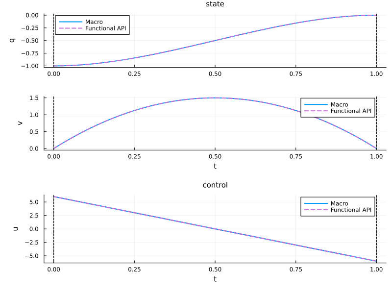
The two models are functionally equivalent. The key difference is visible via definition: the macro records the full DSL expression, whereas the functional API stores an empty definition.

definition(ocp_macro)

Abstract definition:

    t ∈ [t0, tf], time
    x = ((q, v) ∈ R², state)
    u ∈ R, control
    x(t0) == x0
    x(tf) == xf
    ẋ(t) == [v(t), u(t)]
    0.5 * ∫(u(t) ^ 2) → min

has_abstract_definition(ocp_func)

false

Shapes in callbacks

The control above is declared with control!(pre, 1) — dimension 1 — and inside the callbacks f_energy! and lagrange_energy it is used as a bare u, not u[1]. This is not a special case: 1-D state, control and variable components arrive as scalars in every functional-API callback (dynamics!, objective!, constraint!), exactly as on a solution and exactly as the @def convention (see the note on Control). There is no asymmetry between "inside a callback" and "on a solution" — a dimension-1 quantity is a Real everywhere:

u_macro = control(sol_macro)
u_func  = control(sol_func)
u_macro(t0), u_func(t0)

(5.976095617529882, 5.976095617529882)

typeof(u_macro(t0)), typeof(u_func(t0))

(Float64, Float64)

The in-place output buffer is the one exception: dx (dynamics), val (boundary/path constraints) is always a vector of its declared length, written by index, even when that length is 1 — a scalar cannot be mutated in place:

f!(r, t, x, u, v) = (r[1] = -x + u; nothing)  # r is always a vector; x, u here are scalars

This is the one place on the site where this is spelled out; every other page just follows it.

Order and preconditions

• variable! → before time! when using free-time indices (indf, ind0)

• variable! → before dynamics! and objective!

• dynamics! and objective! → after time! and state!

• control! is optional and, when used, has no ordering constraint of its own beyond needing state! first (component-count validation) — see Problems without a control for what omitting it means.

Equivalence

The abstract and functional forms are not just "meant to agree" — it's a tested contract. test/suite/problems/test_forms_equivalent.jl builds both forms for every problem in the shared test library and asserts they agree on dimensions, traits (is_autonomous, is_variable, is_control_free), time-horizon status, cost, dynamics, and constraint-dimension accessors. The one deliberate difference the test itself asserts: has_abstract_definition is true only for the @def form, as shown above.

See also

• Formulation — the mathematics this API builds.

• Abstract syntax (@def) — the macro alternative.

• Problems without a control — omitting control! entirely.

• Inspect a problem — read a built model back.