Multi-phase flows

An optimal control is often made of several arcs: bang arcs, off arcs, singular or boundary arcs, with possibly a jump of the costate at a junction. Each arc has its own flow, and the flows are concatenated, at the switching times, into one flow.

using OptimalControl
using OrdinaryDiffEqTsit5
using Plots

Concatenating two flows

f1 * (t1, f2) follows f1 until t1, then f2. The result is itself a flow:

f1 = Flow(VectorField(x -> 0))    # ẋ = 0
f2 = Flow(VectorField(x -> 1))    # ẋ = 1

f = f1 * (1, f2)
f(0, 0.0, 2)   # constant until t = 1, then one unit of slope 1

0.9999999999999998

More arcs are added the same way: f1 * (t1, f2) * (t2, f3).

Jumps

A jump at the switching time is given between the time and the second flow. On a flow of the state, f1 * (t1, j, f2) applies x ← j(x), or x ← x + j when j is a vector:

fj = f1 * (1, x -> x + 10, f2)
fj(0, 0.0, 2)   # +10 at t = 1, then one unit of slope 1

11.0

On a Hamiltonian flow, the state and the costate are integrated together, and a jump can act on either:

• h1 * (t1, j_x, j_p, h2) applies j_x to the state and j_p to the costate, each a function, a vector to add, or nothing for no jump;

• h1 * (t1, j, h2) with a vector j is a jump of the costate, p ← p + j: the state is continuous, as at the junctions of a boundary arc (see Constrained arcs);

• h1 * (t1, j, h2) with a function j maps the pair, (x, p) ← j(x, p).

On the extremal of the energy problem, a costate jump of at   leaves the state continuous and shifts from to :

h = Flow(
    PseudoHamiltonian((x, p, u) -> p[1] * x[2] + p[2] * u - u^2 / 2),
    DynClosedLoop((x, p) -> p[2]),
)
h_jump = h * (0.5, [10, 0], h)
traj = h_jump((0, 1), [-1, 0], [12, 6])
state(traj)(0.5 - 1e-9) ≈ state(traj)(0.5 + 1e-9), costate(traj)(0.25), costate(traj)(0.75)

(true, [12.0, 3.0000000000000004], [22.0, -5.499999999999997])

Inspecting a concatenation

n_phases(f), get_switching_times(f), get_flow(f, 1) === f1

(2, Real[1], true)

get_flows, get_switching_time(f, i), get_jump(f, i) and get_jumps(f) read back the other parts.

The point call returns one vector

A concatenation is called like any flow: f((t0, tf), x0, p0) for the trajectory, and f(t0, x0, p0, tf) for the final point, with variable= on a problem with a variable. One difference: on Hamiltonian flows, the point call of a concatenation returns one vector [x; p], where a single flow returns the pair (x, p) (CTFlows#439). Write zf = f(…), then zf[1:n] for the state and zf[n+1:2n] for the costate.

Example: minimum time, bang–bang

Minimise for  ,   , from    to . With   ,    is maximised by  . Here is constant and   , so there is one switch, where vanishes. By symmetry it happens at , and the target gives  ,  . The transversality condition   for the Mayer cost (see Notation and conventions), at    and  , gives   , so  .

ocp = @def begin
    tf ∈ R, variable
    t ∈ [0, tf], time
    x = (q, v) ∈ R², state
    u ∈ R, control
    -1 ≤ u(t) ≤ 1
    x(0) == [-1, 0]
    x(tf) == [0, 0]
    ẋ(t) == [v(t), u(t)]
    tf → min
end

f_plus = Flow(ocp, (x, p, v) -> 1)
f_minus = Flow(ocp, (x, p, v) -> -1)

t1, tf = 1, 2
f_bb = f_plus * (t1, f_minus)
zf = f_bb(0, [-1, 0], [1, 1], tf; variable=tf)
xf, pf = zf[1:2], zf[3:4]

([-2.313802281140895e-16, -3.425505599574657e-17], [1.0, -0.9999999999999997])

The concatenation reaches the target, with   .

Example: off arc, then bang

This example comes from the v2.0.4 manual. Minimise the norm of the control, , for    ,   , from    to  :

t0, tf1 = 0, 1
x0, xf1 = -1, 0

ocp_l1 = @def begin
    t ∈ [t0, tf1], time
    x ∈ R, state
    u ∈ R, control
    x(t0) == x0
    x(tf1) == xf1
    -1 ≤ u(t) ≤ 1
    ẋ(t) == -x(t) + u(t)
    ∫(abs(u(t))) → min
end

With   ,      is maximised by   when  , and by   when  . Since  ,  : the control is   (off arc) until reaches , at   , then   (bang arc). Integrating    then     and asking   gives

p0 = 1 / (x0 - (xf1 - 1) * exp(tf1))
t1_l1 = -log(p0)

f_off = Flow(ocp_l1, (x, p) -> 0)    # off arc: u = 0
f_bang = Flow(ocp_l1, (x, p) -> 1)   # bang arc: u = 1

f_l1 = f_off * (t1_l1, f_bang)
sol_l1 = f_l1((t0, tf1), x0, p0)
state(sol_l1)(tf1), objective(sol_l1)

(-3.46276294006056e-11, 0.4586756721429291)

The flow reaches  , and its cost is the length of the bang arc,  :

plot(sol_l1)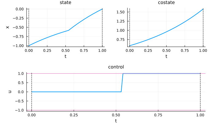

See also

• Constrained arcs: arcs on the boundary of a state constraint, with costate jumps at the junctions.

• Shooting: solve for the switching times and the initial costate, instead of taking them from the analysis as here.

• Time minimisation (bang–bang): the bang–bang example in full.