
Simulation
Sometimes you don't want an optimum — you have a controlled system and a specific control (open-loop or feedback), and you want the trajectory it produces.
using OptimalControl
using OrdinaryDiffEqTsit5
using NLPModelsIpopt
using Plots
The idea
A controlled vector field @def: just ControlledVectorField and a law.
Open loop
fc(x, u) = -x + u

f_ol = Flow(ControlledVectorField(fc), OpenLoop(t -> 1.0))
traj_ol = f_ol((0.0, 1.0), 1.0)
state(traj_ol)(0.5)1.0OpenLoop is unconditionally non-autonomous
The law must be u(t) (or u(t, v) with a variable) — always a function of time, never a bare constant closure. OpenLoop(() -> 1.0) builds without error but fails on the first call, with a bare MethodError far from the actual mistake:
julia> bad_law = OpenLoop(() -> 1.0);   # constructs fine — the trap

julia> Flow(ControlledVectorField(fc), bad_law)(0.0, 1.0, 1.0)
MethodError: no method matching (::Main.var"#5#6")(::Float64)
The anonymous function `#5` exists, but no method is defined for this combination of argument types.

Closest candidates are:
  (::Main.var"#5#6")()
   @ Main REPL[1]:1
OpenLoop(t -> 1.0) above is the only correct spelling — there is no "autonomous open loop" any more. See Migration for the full list of silent v2.0 → v2.1 semantics changes.
Closed loop (feedback)
f_cl = Flow(ControlledVectorField(fc), ClosedLoop(x -> 0.5x))
f_cl(0.0, 1.0, 1.0)0.6065306597356303DynClosedLoop (the costate-carrying law kind) is rejected on a ControlledVectorField — it has no costate to carry:
julia> Flow(ControlledVectorField(fc), DynClosedLoop((x, p) -> x))
PreconditionError → #_flow_from_controlled_vf#48, building.jl:518
│
│  Flow(fc, law) requires an OpenLoop or ClosedLoop control law
│
│  Reason   a DynClosedLoop law u(t,x,p,v) needs the costate p, which a state flow of a vector field does not have
│
│  Context  Flow(fc::ControlledVectorField, law::ControlLaw) — feedback dispatch
│  Hint     use OpenLoop(u) or ClosedLoop(u); for a DynClosedLoop law use Flow(h̃, law) or Flow(ocp, law)
└─
From an optimal control problem
t0 = 0
tf = 1
x0 = [-1, 0]

ocp = @def begin
    t ∈ [t0, tf], time
    x = (q, v) ∈ R², state
    u ∈ R, control
    x(t0) == x0
    x(tf) == [0, 0]
    ẋ(t) == [v(t), u(t)]
    0.5∫(u(t)^2) → min
end

f_sim = Flow(ocp, OpenLoop(t -> 1.0))
traj_ocp = f_sim((t0, tf), x0)
Flow(ocp, OpenLoop(u)) returns a ControlledFlow whose trajectory carries the objective — you can evaluate a candidate control's cost directly:
objective(traj_ocp)0.4999999999999999A flow built without an OCP has no cost to report — calling objective on it is a PreconditionError, not a silent 0.0 or NaN:
julia> objective(traj_ol)
PreconditionError → objective, state_flow_trajectory.jl:310
│
│  this StateFlowTrajectory has no objective value
│
│  Reason   it was built without an optimal control problem (e.g. from Flow(fc, law) rather than Flow(ocp, law)), so there is no cost to evaluate
│
│  Context  StateFlowTrajectory — objective getter
│  Hint     build the flow from an OCP — Flow(ocp, law) — to obtain the objective, or use state(sol) and control(sol)
└─
Inspecting the trajectory
Same accessors as a solve-returned Solution:
state(traj_ocp)(0.5), control(traj_ocp)(0.5), time_grid(traj_ocp)([-0.8749999999999987, 0.5000000000000004], 1.0, [0.0, 0.010717734625362933, 0.1696232142444496, 1.0])Plotting it
plot(traj_ocp)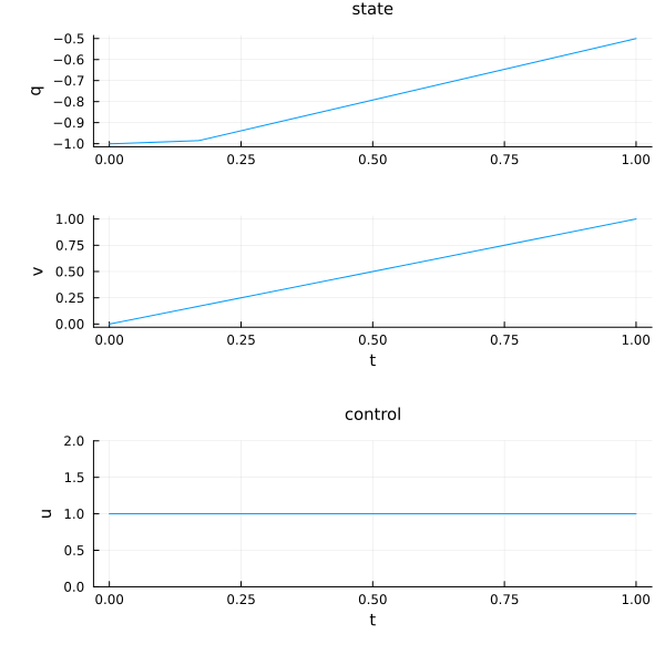
See Plot for every keyword.
Point vs trajectory
f(t0, x0, tf) returns the endpoint only; f((t0, tf), x0) returns the full trajectory — same convention as every other flow in this section.
The trajectory's own type — CTFlows.Trajectories.StateFlowTrajectory — is not re-exported; never name it in your own code, only call the generic accessors on it.
See also
Solution object and Plot — the accessors used above, in full.
From an OCP — the indirect-solving counterpart, where the law comes from the PMP instead of being handed to you.
No control — control-free problems, a related but distinct case.