The logo

The OptimalControl.jl logo is not a drawing. It is the solution of an optimal control problem — an energy-minimal low-thrust orbit transfer — solved once and repeated by symmetry.

A spacecraft spirals from a low circular orbit out to a higher one under continuous weak thrust. Two-body dynamics do not care which way is up, so the same optimal transfer, rotated by  , gives three trajectories at once — and their three departure points sit exactly where the three dots of the Julia logo go, winding onto the outer orbit around the central body.

This page rebuilds that figure from scratch.

The transfer problem

Normalised two-body dynamics (gravitational parameter  ). The state is the spacecraft's position and velocity in the orbital plane,

and the control   is the thrust acceleration. The spacecraft starts on a circular orbit of radius and must reach a circular orbit of radius : at the final time it has to be at the right radius, at the right (circular) speed, and with zero radial velocity — the final angular position is free. Along the way it minimises the thrust energy .

using OptimalControl
using NLPModelsIpopt

r0 = 1.1      # departure orbit radius
rf = 2.2      # target orbit radius
tf = 2π       # transfer duration — sets how far the trajectory winds

ocp = @def begin
    t ∈ [0, tf], time
    x ∈ R⁴,      state
    u ∈ R²,      control

    x(0) == [r0, 0, 0, 1 / sqrt(r0)]          # circular orbit of radius r0

    x₁(tf)^2 + x₂(tf)^2 == rf^2               # insertion radius
    x₃(tf)^2 + x₄(tf)^2 == 1 / rf             # circular speed at radius rf
    x₁(tf) * x₃(tf) + x₂(tf) * x₄(tf) == 0    # zero radial velocity

    ẋ(t) == [ x₃(t),
              x₄(t),
             -x₁(t) / (x₁(t)^2 + x₂(t)^2)^(3 / 2) + u₁(t),
             -x₂(t) / (x₁(t)^2 + x₂(t)^2)^(3 / 2) + u₂(t) ]

    ∫(u₁(t)^2 + u₂(t)^2) → min
end

Abstract definition:

    t ∈ [0, tf], time
    x ∈ R⁴, state
    u ∈ R², control
    x(0) == [r0, 0, 0, 1 / sqrt(r0)]
    x₁(tf) ^ 2 + x₂(tf) ^ 2 == rf ^ 2
    x₃(tf) ^ 2 + x₄(tf) ^ 2 == 1 / rf
    x₁(tf) * x₃(tf) + x₂(tf) * x₄(tf) == 0
    ẋ(t) == [x₃(t), x₄(t), -(x₁(t)) / (x₁(t) ^ 2 + x₂(t) ^ 2) ^ (3 / 2) + u₁(t), -(x₂(t)) / (x₁(t) ^ 2 + x₂(t) ^ 2) ^ (3 / 2) + u₂(t)]
    ∫(u₁(t) ^ 2 + u₂(t) ^ 2) → min

The (autonomous) optimal control problem is of the form:

    minimize  J(x, u) = ∫ f⁰(x(t), u(t)) dt, over [0, 6.28]

    subject to

        ẋ(t) = f(x(t), u(t)), t in [0, 6.28] a.e.,

        ϕ₋ ≤ ϕ(x(0), x(6.28)) ≤ ϕ₊, 

    where x(t) ∈ R⁴ and u(t) ∈ R².

Solving it

Low-thrust transfers are hard to solve from a cold start, so we warm-start with a crude analytical spiral: let the radius grow linearly from to and advance the angle at the local Keplerian rate  . (More on initial guesses in Initial guess.)

k = (rf - r0) / tf

function spiral_guess(t)
    r  = r0 + k * t
    θ  = (2 / k) * (1 / sqrt(r0) - 1 / sqrt(r))
    dθ = r^(-3 / 2)
    return [r * cos(θ), r * sin(θ),
            k * cos(θ) - r * dθ * sin(θ), k * sin(θ) + r * dθ * cos(θ)]
end

sol = solve(ocp; grid_size = 400, display = false,
            init = (state = spiral_guess, control = t -> [0, 0]))

xf = state(sol)(tf)
(insertion_radius = sqrt(xf[1]^2 + xf[2]^2),
 insertion_speed  = sqrt(xf[3]^2 + xf[4]^2),
 radial_velocity  = xf[1] * xf[3] + xf[2] * xf[4],
 thrust_energy    = objective(sol))

(insertion_radius = 2.200000000045782, insertion_speed = 0.6741998624766782, radial_velocity = -2.2457036230605354e-12, thrust_energy = 0.03520813302745113)

The insertion radius and speed reach their targets and the radial velocity is zero: the spacecraft arrives tangent to the outer orbit.

Looking at the solution

The site's documentation renders solution plots with Plots.jl; here we use the Makie backend instead — load a Makie package and the Makie.plot method for a solution becomes available.

using CairoMakie

Makie.plot(sol)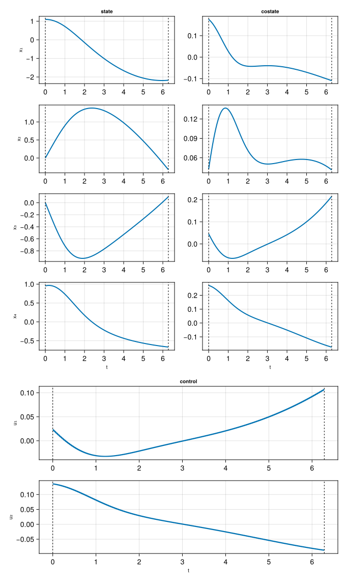

The thrust () stays small throughout — this is a low-thrust transfer, nudging the orbit rather than forcing it. The right-hand column is the costate, the adjoint of Pontryagin's Maximum Principle, which the solver returns alongside the state and control.

The trajectory in the plane

The logo lives in the plane. One transfer is a single spiral from the inner orbit to the outer one.

xt  = state(sol)
arc = [Point2f(xt(t)[1], xt(t)[2]) for t in range(0, tf; length = 500)]

circle(r) =
    [Point2f(r * cos(a), r * sin(a)) for a in range(0, 2π; length = 300)]

fig = Figure(size = (460, 460))
ax  = Axis(fig[1, 1]; aspect = DataAspect())
lines!(ax, circle(r0); color = (:gray, 0.5))
lines!(ax, circle(rf); color = (:gray, 0.5))
lines!(ax, arc;        color = :purple, linewidth = 3)
scatter!(ax, arc[1];   color = :purple, markersize = 14)
fig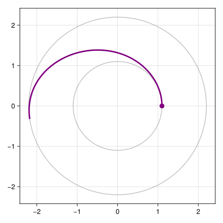

Three-fold symmetry

Two-body dynamics are rotation-equivariant: if   is an optimal transfer, so is the whole trajectory rotated by any fixed angle — same cost, same constraints. Rotating the solved spiral by and gives three transfers for the price of one.

Colour them with the Julia logo palette, drop a dot at each departure point, add the target orbit in Julia blue and the central body, and the logo is done.

using Colors

rot(ψ) = [cos(ψ) -sin(ψ); sin(ψ) cos(ψ)]
jl = Colors.JULIA_LOGO_COLORS   # (red, green, blue, purple)

# departure points placed as the Julia-logo dots — green on top
arms = [(7π / 6, jl.red), (π / 2, jl.green), (11π / 6, jl.purple)]

fig = Figure(size = (600, 600), backgroundcolor = :transparent)
ax  = Axis(
    fig[1, 1];
    aspect = DataAspect(), backgroundcolor = :transparent,
)
hidedecorations!(ax)
hidespines!(ax)
limits!(ax, -1.32rf, 1.32rf, -1.32rf, 1.32rf)

poly!(ax, circle(rf); color = :white)   # white disk behind everything

for (ψ, c) in arms
    P = [Point2f(rot(ψ) * p) for p in arc]
    lines!(ax, P; color = c, linewidth = 13)
    scatter!(ax, P[1]; color = :white, markersize = 80)   # halo
    scatter!(ax, P[1]; color = c,      markersize = 60)   # coloured dot
end

lines!(ax, circle(rf); color = jl.blue, linewidth = 13)   # target orbit
scatter!(ax, Point2f(0, 0); color = :white,  markersize = 50)
scatter!(ax, Point2f(0, 0); color = jl.blue, markersize = 100)

fig

That is the figure the site uses as its logo (docs/src/assets/logo.png).

The published asset is produced by a slightly more elaborate script — crisper strokes, a few tuning knobs — kept in the repository at .extras/logos/logo-gagnant/. The optimal control problem it solves is exactly the one above.

See also

• Initial guess — the warm-start used here, and the others.

• Plot — the Plots backend, and what a solution plot shows.

• Example gallery — the other worked problems.