
Parameter estimation without a control
Two problems with no control anywhere — only a variable to fit to data. See No control for the modelling side of this; this page is the full worked story, direct and indirect, for both.
using OptimalControl
using NLPModelsIpopt
using OrdinaryDiffEqTsit5
using NonlinearSolve
using Plots
Growth-rate estimation
The problem
Fit
Definition
λ_true = 0.5
x_true(t) = 2 * exp(λ_true * t)
data(t) = x_true(t) + 0.2 * sin(4π * t)

t0 = 0
tf = 2
x0 = 2

ocp_growth = @def begin
    λ ∈ R, variable
    t ∈ [t0, tf], time
    x ∈ R, state

    x(t0) == x0

    ẋ(t) == λ * x(t)

    ∫((x(t) - data(t))^2) → min
end
Abstract definition:
λ ∈ R, variable
t ∈ [t0, tf], time
x ∈ R, state
x(t0) == x0
ẋ(t) == λ * x(t)
∫((x(t) - data(t)) ^ 2) → min
The (non autonomous) optimal control problem is of the form:
minimize J(x, λ) = ∫ f⁰(t, x(t), λ) dt, over [0, 2]
subject to
ẋ(t) = f(t, x(t), λ), t in [0, 2] a.e.,
ϕ₋ ≤ ϕ(x(0), x(2), λ) ≤ ϕ₊,
where x(t) ∈ R and λ ∈ R.Direct solution
growth_sol = solve(ocp_growth; grid_size=20, display=false)
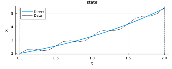
println("estimated λ = ", variable(growth_sol))
estimated λ = 0.4960778956661449t_grid = time_grid(growth_sol)
plt_growth = plot(growth_sol, :state; label="Direct")
plot!(
plt_growth, t_grid, data.(t_grid);
line=:dot, label="Data", color=:black,
)
model(growth_sol) gives back the underlying problem the solution was computed from — the same object ocp_growth was build-ed into:
model(growth_sol) === ocp_growthtrueIndirect solution
The pseudo-Hamiltonian is
f_growth = Flow(ocp_growth)OptimalControlFlow
├─ system: HamiltonianSystem
│ ├─ time_dependence: NonAutonomous
│ ├─ variable_dependence: NonFixed
│ ├─ Hamiltonian: non-autonomous, variable
│ │ natural call: h(t, x, p, v)
│ │ uniform call: h(t, x, p, v)
│ └─ backend: DifferentiationInterface{CPU}(ad_backend=AutoForwardDiff)
└─ integrator: SciML{CPU} (instance, id=:sciml)
├─ internalnorm = real_norm [default]
├─ alg = Tsit5 [default]
├─ reltol = 1.0e-8 [default]
├─ save_everystep = auto [default]
├─ abstol = 1.0e-8 [default]
├─ save_start = auto [default]
└─ dense = auto [default]
Tip: use describe(SciML{CPU}) to see all available options.The costate
function shoot_growth!(s, ξ)
    p0, λ = ξ[1], ξ[2]
    _, p_tf, pλ_tf = f_growth(
        t0, x0, p0, tf; variable=λ, variable_costate=true
    )
    s[1] = p_tf
    s[2] = pλ_tf
    return nothing
end
shoot_growth! (generic function with 1 method)nle_growth!(s, ξ, _) = shoot_growth!(s, ξ)
p0_guess = costate(growth_sol)(t0)
λ_guess = variable(growth_sol)
prob_growth = NonlinearProblem(nle_growth!, [p0_guess, λ_guess])
shoot_sol_growth = NonlinearSolve.solve(prob_growth; show_trace=Val(false))
p0_sol_growth, λ_sol = shoot_sol_growth.u2-element Vector{Float64}:
0.05847851053034825
0.4966212669628472Comparison
indirect_growth = f_growth((t0, tf), x0, p0_sol_growth; variable=λ_sol)
plot!(
    plt_growth, indirect_growth, :state;
    label="Indirect", linestyle=:dash,
)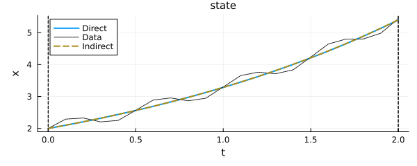
The direct and indirect estimates of
Harmonic-oscillator pulsation
The problem
,
Definition
q0 = 1
v0 = 0
t0h = 0
tfh = 1

ocp_harmonic = @def begin
    ω ∈ R, variable
    t ∈ [t0h, tfh], time
    x = (q, v) ∈ R², state

    q(t0h) == q0
    v(t0h) == v0
    q(tfh) == 0.0

    ẋ(t) == [v(t), -ω^2 * q(t)]

    ω^2 → min
end
Abstract definition:
ω ∈ R, variable
t ∈ [t0h, tfh], time
x = ((q, v) ∈ R², state)
q(t0h) == q0
v(t0h) == v0
q(tfh) == 0.0
ẋ(t) == [v(t), -(ω ^ 2) * q(t)]
ω ^ 2 → min
The (autonomous) optimal control problem is of the form:
minimize J(x, ω) = g(x(0), x(1), ω)
subject to
ẋ(t) = f(x(t), ω), t in [0, 1] a.e.,
ϕ₋ ≤ ϕ(x(0), x(1), ω) ≤ ϕ₊,
where x(t) = (q(t), v(t)) ∈ R² and ω ∈ R.Direct solution
harmonic_sol = solve(ocp_harmonic; grid_size=20, display=false)
println(
    "estimated ω = ", variable(harmonic_sol),
    "  (expected π/2 ≈ ", π / 2, ")",
)
estimated ω = 1.5716042803951324 (expected π/2 ≈ 1.5707963267948966)plot(harmonic_sol, :state; label="Direct")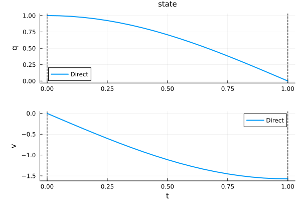
Indirect solution
f_harmonic = Flow(ocp_harmonic)

function shoot_harmonic!(s, ξ)
    p0, ω = ξ[1:2], ξ[3]
    x_tf, p_tf, pω_tf = f_harmonic(
        t0h, [q0, v0], p0, tfh; variable=ω, variable_costate=true
    )
    s[1] = x_tf[1]           # q(tf) = 0
    s[2] = p_tf[2]           # free final velocity
    s[3] = pω_tf + 2ω        # Mayer-cost transversality
    return nothing
end
shoot_harmonic! (generic function with 1 method)nle_harmonic!(s, ξ, _) = shoot_harmonic!(s, ξ)
p0_guess_h = costate(harmonic_sol)(t0h)
ω_guess = variable(harmonic_sol)
prob_harmonic = NonlinearProblem(nle_harmonic!, [p0_guess_h..., ω_guess])
shoot_sol_harmonic = NonlinearSolve.solve(
prob_harmonic; show_trace=Val(false)
)
p0_sol_harmonic, ω_sol = shoot_sol_harmonic.u[1:2], shoot_sol_harmonic.u[3]
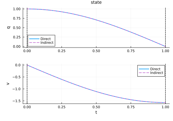
println("indirect ω = ", ω_sol)indirect ω = 1.570796326752619Comparison
indirect_harmonic = f_harmonic(
    (t0h, tfh), [q0, v0], p0_sol_harmonic; variable=ω_sol
)
plt_harmonic = plot(harmonic_sol, :state; label="Direct")
plot!(
    plt_harmonic, indirect_harmonic, :state;
    label="Indirect", linestyle=:dash,
)
See also
No control — the modelling-side guide for control-free problems.
Control and variable together — the same two systems, with a control added back in.
From an OCP — control-free flows (
Flow(ocp), no law), in general.