
Time minimisation (bang–bang)
Same wagon as Energy minimisation, but transferred as fast as possible instead of at minimal energy — a bounded control gives a bang–bang optimal law with a single switch.
using OptimalControl
using NLPModelsIpopt
using OrdinaryDiffEqTsit5
using NonlinearSolve
using Plots
The problem
Same dynamics,
Definition
t0 = 0
x0 = [-1, 0]
xf = [0, 0]

ocp = @def begin
    tf ∈ R, variable
    t ∈ [t0, tf], time
    x = (q, v) ∈ R², state
    u ∈ R, control

    -1 ≤ u(t) ≤ 1

    x(t0) == x0
    x(tf) == xf

    ẋ(t) == [v(t), u(t)]

    tf → min
end
Abstract definition:
tf ∈ R, variable
t ∈ [t0, tf], time
x = ((q, v) ∈ R², state)
u ∈ R, control
-1 ≤ u(t) ≤ 1
x(t0) == x0
x(tf) == xf
ẋ(t) == [v(t), u(t)]
tf → min
The (autonomous) optimal control problem is of the form:
minimize J(x, u, tf) = g(x(0), x(tf), tf)
subject to
ẋ(t) = f(x(t), u(t), tf), t in [0, tf] a.e.,
ϕ₋ ≤ ϕ(x(0), x(tf), tf) ≤ ϕ₊,
u₋ ≤ u(t) ≤ u₊,
where x(t) = (q(t), v(t)) ∈ R², u(t) ∈ R and tf ∈ R.Direct solution
direct_sol = solve(ocp; grid_size=20, display=false)
plt = plot(direct_sol, :state, :control; label="Direct")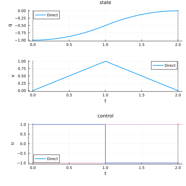
Indirect solution
The pseudo-Hamiltonian
H(x, p, u) = p[1] * x[2] + p[2] * u - 1

u_max = 1.0
u_min = -1.0

f_max = Flow(ocp, (x, p, v) -> u_max)
f_min = Flow(ocp, (x, p, v) -> u_min)
OptimalControlFlow
├─ system: HamiltonianSystem
│ ├─ time_dependence: Autonomous
│ ├─ variable_dependence: NonFixed
│ ├─ ComposedHamiltonian: autonomous, variable
│ │ natural call: h(x, p, v)
│ │ uniform call: h(t, x, p, v)
│ └─ backend: DifferentiationInterface{CPU}(ad_backend=AutoForwardDiff)
└─ integrator: SciML{CPU} (instance, id=:sciml)
├─ internalnorm = real_norm [default]
├─ alg = Tsit5 [default]
├─ reltol = 1.0e-8 [default]
├─ save_everystep = auto [default]
├─ abstol = 1.0e-8 [default]
├─ save_start = auto [default]
└─ dense = auto [default]
Tip: use describe(SciML{CPU}) to see all available options.The free final time makes this a NonFixed flow: every call needs variable=.
function shoot!(s, ξ)
    p0 = ξ[1:2]
    t1, tf = ξ[3], ξ[4]

    x1, p1 = f_max(t0, x0, p0, t1; variable=tf)
    xf_, pf = f_min(t1, x1, p1, tf; variable=tf)

    s[1:2] = xf_ - xf     # target reached
    s[3] = p1[2]          # switching condition
    s[4] = H(xf_, pf, u_min)  # free final time transversality
    return nothing
end
shoot! (generic function with 1 method)nle!(s, ξ, _) = shoot!(s, ξ)
p0_guess = costate(direct_sol)(t0)
t1_guess = 0.9 * variable(direct_sol)
tf_guess = variable(direct_sol)
ξ_guess = [p0_guess..., t1_guess, tf_guess]
prob = NonlinearProblem(nle!, ξ_guess)
shooting_sol = NonlinearSolve.solve(prob; show_trace=Val(false))
p0_sol, t1_sol, tf_sol =
shooting_sol.u[1:2], shooting_sol.u[3], shooting_sol.u[4]([0.9999999999999966, 1.0], 1.0000000000000002, 2.000000000000001)s = zeros(4)
shoot!(s, shooting_sol.u)
s4-element Vector{Float64}:
2.905637696828105e-16
-4.790704380274452e-16
3.644464827880472e-15
-7.105427357601002e-15Comparison
Concatenating the two constant-control flows at the switching time reconstructs the whole trajectory:
φ = f_max * (t1_sol, f_min)
indirect_sol = φ((t0, tf_sol), x0, p0_sol; variable=tf_sol)
plot!(plt, indirect_sol, :state, :control; label="Indirect")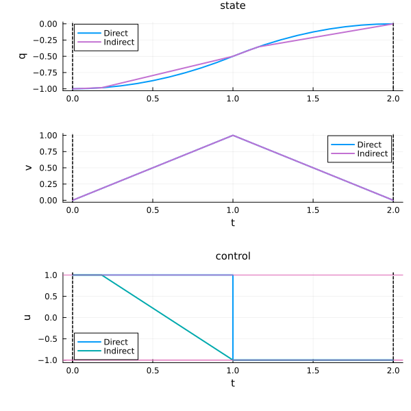
See also
Multi-phase flows — flow concatenation
*, in general.Shooting — bang–bang shooting, worked in full detail from this exact problem.
Energy minimisation — the same wagon, unbounded control.