Getting Started

This page gets you from installation to your first integrated trajectory in five minutes.

Installation

import Pkg
Pkg.add("CTFlows")

To integrate anything you also need an ODE solver backend. The default strategy is SciML, activated by loading an OrdinaryDiffEq solver package:

Pkg.add("OrdinaryDiffEqTsit5")

Mental model

Three ideas explain most of the API: 2. No top-level exports. CTFlows exports nothing at the package level. Every symbol lives in a submodule and is reached via a qualified path (CTFlows.Flows.Flow) or an explicit using CTFlows.Flows. The same holds for the data layer, which lives in CTBase (CTBase.Data.VectorField).

3. A pipeline of small layers. Data (your functions, wrapped) → Systems (ODE right-hand side) → Integrators (solver strategy) → Flows (the callable object) → Trajectories (the result). The shortcut Flows.Flow(data; opts...) runs the whole pipeline in one call.

4. Extension-backed features. The actual ODE solving, plotting, and SciML interoperability are Julia package extensions: they activate when you load OrdinaryDiffEqTsit5 (or another solver), Plots, or SciMLBase.

5-minute walkthrough

Bring the relevant submodules into scope and load a solver:

using CTFlows
using CTBase.Data          # VectorField, Hamiltonian, HamiltonianVectorField
using CTFlows.Flows        # Flow
using CTFlows.Trajectories # time_grid, state, costate
import OrdinaryDiffEqTsit5 # activates the SciML integrator extension

Wrap the dynamics

A vector field is any function of the state. Wrapping it as a Data.VectorField records its traits (autonomous or not, with or without a variable parameter):

vf = Data.VectorField(x -> -x)   # autonomous, fixed

Build the flow

flow = Flows.Flow(vf; reltol=1e-8, abstol=1e-8)

Flow
├─ system: VectorFieldSystem
│          ├─ wraps: VectorField: autonomous, fixed (no variable), out-of-place
│          └─ rhs: IPVFOoPRHS (out-of-place VF → in-place interface)
└─ integrator: SciML (abstol = 1.0e-8, reltol = 1.0e-8)

Integrate

Point form returns only the final state:

julia> xf = flow(0.0, [1.0, 0.0], 1.0)
2-element Vector{Float64}:
 0.36787944127643124
 0.0

Trajectory form returns the full history:

sol = flow((0.0, 1.0), [1.0, 0.0])

VectorFieldTrajectory
├─ result: SciMLIntegrationResult
├─ tspan: (0.0, 1.0)
├─ time points: 16
└─ final state: [0.36787944127643124, 0.0]

Read the result

julia> ts = Trajectories.time_grid(sol);

julia> (ts[1], ts[end])
(0.0, 1.0)

julia> x = Trajectories.state(sol);

julia> x(0.5)
2-element Vector{Float64}:
 0.6065306592843308
 0.0

Trajectories.state(sol) is callable and interpolates: x(t) gives the state at any t inside the integration interval.

Hamiltonian systems

The same API drives Hamiltonian dynamics on state–costate pairs :

hvf = Data.HamiltonianVectorField((x, p) -> (p, -x))
hflow = Flows.Flow(hvf; reltol=1e-10)

julia> xf, pf = hflow(0.0, [1.0, 0.0], [0.0, 1.0], 1.0);

julia> xf
2-element Vector{Float64}:
 0.5403023057842606
 0.8414709847533869

julia> pf
2-element Vector{Float64}:
 -0.8414709847533869
  0.5403023057842606

You can also start from a scalar Hamiltonian and let automatic differentiation derive the vector field — see Building a flow.

Optimal control problems

This is the entry point most users of the control-toolbox ecosystem actually reach for: Flow(ocp) builds a flow directly from an optimal control problem — a CTModels.Models.Model — with no Hamiltonian to write by hand.

using CTModels

pre = CTModels.Building.PreModel()
CTModels.Building.time_dependence!(pre; autonomous=true)
CTModels.Building.time!(pre; t0=0.0, tf=1.0)
CTModels.Building.state!(pre, 1)
CTModels.Building.dynamics!(pre, (r, t, x, u, v) -> (r[1] = -x[1]; nothing))
CTModels.Building.objective!(pre, :min; mayer=(x0, xf, v) -> xf[1])
ocp = CTModels.Building.build(pre)

f = Flows.Flow(ocp; reltol=1e-10)

Point evaluation returns the final state–costate pair (Hamiltonian semantics):

julia> xf, pf = f(0.0, [1.0], [1.0], 1.0);

julia> xf
0.3678794412026476

julia> pf
2.718281828560478

A trajectory call assembles a full CTModels.Solution — state, costate, and the objective value:

sol = f((0.0, 1.0), [1.0], [1.0])

Solution  ✓ successful
  │  Objective : 0.36787944120264765
  │  Status : Success
  └─ Message : Solution computed by CTFlows OCP flow

julia> CTModels.Components.objective(sol)
0.36787944120264765

This is a control-free problem (no u in the dynamics). For a problem with a control, pass a control law — Flow(ocp, law) — see Control laws. See Optimal control for the full picture, including the basic no-costate call f(t0, x0, tf) for direct shooting.

Plotting the result

Load Plots and any solution object draws directly — here the state and costate of the CTModels.Solution on a shared time axis:

plot(sol)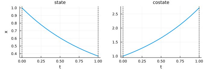

Where to go next

• Optimal control — flows built directly from a CTModels problem.

• Control laws — Flow(ocp, law), OpenLoop / ClosedLoop / DynClosedLoop.

• Flows overview — the full pipeline and the mathematical setting.

• Integrating — call styles, variable parameters, solver options.

• Multi-phase flows — concatenation with switching times and jumps.

• SciML flows — wrap an existing ODEFunction or ODEProblem.