Constrained flows
Flow(ocp, law; constraint, multiplier) augments the pseudo-Hamiltonian with a path constraint term, for OCPs whose Pontryagin's Maximum Principle carries a state or mixed constraint alongside the control. This chapter covers the API, the sign convention, the hamiltonian_type semantics for constrained flows (:total vs :partial, and why they agree on a constrained arc), and two worked examples.
The augmented pseudo-Hamiltonian
Given the OCP's own pseudo-Hamiltonian
Pass constraint/multiplier to Flow(ocp, law; …) alongside a DynClosedLoop law — they must be given together:
# OCP: ẋ = -x + u, min ∫ 0.5*u^2 dt  (autonomous, fixed, 1-D — scalar convention)
pre = CTModels.Building.PreModel()
CTModels.Building.time_dependence!(pre; autonomous=true)
CTModels.Building.time!(pre; t0=0.0, tf=1.0)
CTModels.Building.state!(pre, 1)
CTModels.Building.control!(pre, 1)
CTModels.Building.dynamics!(pre, (r, t, x, u, v) -> (r[1] = -x + u; nothing))
CTModels.Building.objective!(pre, :min; lagrange=(t, x, u, v) -> 0.5 * u^2)
ocp = CTModels.Building.build(pre)

law = Data.DynClosedLoop((x, p) -> p)   # u = p (from ∂H̃/∂u = p - u = 0)
c = 0.3
f = Flows.Flow(
    ocp, law;
    constraint=Data.StateConstraint(x -> x),
    multiplier=Data.Multiplier((x, p) -> c),
    reltol=1e-10,
)
A raw Function is accepted directly for constraint/multiplier (wrapped in a MixedConstraint/Multiplier with the OCP's own time/variable dependence, just like Flow(ocp, u::Function) — see Control laws):
f2 = Flows.Flow(ocp, law; constraint=(x, u) -> x, multiplier=(x, p) -> c, reltol=1e-10)
xf, pf = f2(0.0, 1.0, 0.5, 1.0)
xf, pf
(0.7925558476344876, 0.8436563657430431)A labelled :path constraint from the OCP itself also resolves — pass its Symbol label as constraint.
Sign convention
Flow(ocp, law; constraint, multiplier) uses
Under g ≥ 0, the multiplier is
Multiple constraints
A single constraint carrier — a :path label or a raw function — can already be vector-valued (returning a vector, paired with a vector multiplier): the
To combine separately-defined constraints, pass tuples of matched length:
g1(x, u) = x
g2(x, u) = 1.0 - x
μ1(x, p) = 0.4
μ2(x, p) = 0.1
ft = Flows.Flow(ocp, law; constraint=(g1, g2), multiplier=(μ1, μ2), reltol=1e-10)
Each gᵢ/μᵢ is resolved independently (raw functions, :path labels, or explicit carriers can be mixed within the tuple); the flow sums Flow throws a CTBase.Exceptions.IncorrectArgument.
hamiltonian_type for constrained flows
The hamiltonian_type keyword (:total default, :partial) works as for unconstrained flows (see Control laws), extended to the constraint term:
:total: composewith the law into a CTBase.Data.ComposedHamiltonianand differentiate through the law and the multiplier (total derivative in, , ). :partial: freeze both the controlis differentiated in , is not.
ft_ = Flows.Flow(
    ocp, law; constraint=Data.StateConstraint(x -> x),
    multiplier=Data.Multiplier((x, p) -> c), hamiltonian_type=:total, reltol=1e-10,
)
fp_ = Flows.Flow(
    ocp, law; constraint=Data.StateConstraint(x -> x),
    multiplier=Data.Multiplier((x, p) -> c), hamiltonian_type=:partial, reltol=1e-10,
)
x0, p0, tf = 1.0, 0.5, 1.0
ft_(0.0, x0, p0, tf), fp_(0.0, x0, p0, tf)   # constant μ, stationary law ⇒ agree
((0.7925558476344876, 0.8436563657430431), (0.7925558476344876, 0.8436563657430431))Why :total and :partial agree on a constrained arc
Pontryagin's Maximum Principle with a state constraint
:partial is exactly :total adds the two extra chain-rule terms. Both vanish on the arc:
; order 2: a richer invariant), or because
So :total and :partial coincide on a constrained arc, and a shooting method's entry conditions put the trajectory exactly there — this is why both modes converge to the same solution in practice, as the two worked examples below demonstrate.
Plotting a constrained trajectory
A constrained Flow(ocp, law; constraint, multiplier) with a DynClosedLoop law is an OptimalControlFlow, so a trajectory call returns a CTModels.Solution with the control reconstructed from the law — plot it directly once Plots is loaded:
sol = f((0.0, 1.0), 1.0, 0.5)   # trajectory call on the constrained flow f
plot(sol)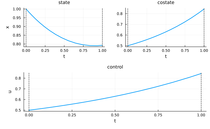
Worked example: Goddard problem (order 1)
The Goddard rocket problem (maximise final mass under a velocity path constraint, free final time) has four arcs — two bang arcs (:total and :partial converge, from the known solution and from a perturbed Newton restart, to the same shooting solution (residual < 1e-7 in both modes). This is also an end-to-end integration test of the whole convenience surface — raw-function control law, raw-function constraint (MixedConstraint, NonFixed free final time — built directly from a CTModels.Model and rebuilt across all four arcs with Flow(ocp, law; constraint, multiplier), then reconstructed across phases with the * multi-phase operator (see Multi-phase flows) into a single CTModels.Solution. See test/suite/integration/test_goddard_ocp.jl in the repository.
Worked example: double integrator (order 2)
The time-minimal double integrator with a second-order position constraint H_1\,u_c' vanishes because :total ≡ :partial equivalence. The costate jumps at the two junctions between the interior and boundary arcs (f1 * (t1, jump, f2), see Multi-phase flows), and the reconstructed multi-phase solution's control is exactly test/suite/integration/test_double_integrator_state.jl.
See also
CTFlows.Flows.Flow(ocp::CTModels.Models.Model, law::CTBase.Data.ControlLaw)— the constructor acceptingconstraint/multiplier.CTFlows.Flows._resolve_constraint,CTFlows.Flows._resolve_multiplier— spec resolution (label, carrier, function, tuple).CTBase.Data.StateConstraint,CTBase.Data.ControlConstraint,CTBase.Data.MixedConstraint,CTBase.Data.Multiplier— explicit constructors.Control laws —
hamiltonian_type, the raw-function convenience.Multi-phase flows —
*concatenation, costate jumps.Optimal control — the unconstrained pseudo-Hamiltonian.