Multi-phase flows
A multi-phase flow concatenates several single-phase flows end-to-end, with switching times between phases and optional jump functions applied at each switch. The integration is exact: each phase is solved independently, and the output of one phase becomes the initial condition of the next.
Concatenation operator *
Use the * operator to chain two flows at a switching time:
# flow1 on [t0, 1.0], then flow2 on [1.0, tf]
mpf = flow1 * (1.0, flow2)
MultiPhaseStateFlow
├─ phases: 2
├─ systems: VectorFieldSystem, VectorFieldSystem
├─ integrators: SciML, SciML
├─ switching_times: Real[1.0]
└─ jumps: Any[nothing]The result is a MultiPhaseStateFlow. You can chain more phases:
mpf3 = flow1 * (0.5, flow2) * (1.0, flow3)
MultiPhase.n_phases(mpf3)3Switching times must be strictly increasing. If they are not, a PreconditionError is thrown.
Phases with different dynamics
Each phase may wrap a different vector field — the dynamics, system type, and integrator are all free per phase. The only requirement is that all phases share the same TimeDependence and VariableDependence traits (both autonomous or both non-autonomous, both fixed or both variable).
# flow1: f(x) = -x   |   flow_het: f(x) = -2x  — different functions, same TD/VD
mpf_het = flow1 * (1.0, flow_het)
MultiPhase.n_phases(mpf_het)2This enables the typical use cases of multi-phase optimal control:
Bang-bang trajectories:
flow_plus * (t_switch, flow_minus)with distinct controlled dynamics per arc.Multi-regime systems: phases with different physical models (e.g. free flight / contact phase).
Different solvers per phase: stiff phases can use an implicit integrator while smooth phases use an explicit one.
Mixing state flows with Hamiltonian flows is not allowed — attempting it raises a PreconditionError.
Jumps at switching times
An additive vector jump_x is added to the state at the switching time (x ← x + jump_x). Pass it as the second element of the switching tuple:
jump_x = [0.5, 0.0]   # add 0.5 to the first component at the switch

mpf_jump = flow1 * (1.0, jump_x, flow2)
MultiPhaseStateFlow
├─ phases: 2
├─ systems: VectorFieldSystem, VectorFieldSystem
├─ integrators: SciML, SciML
├─ switching_times: Real[1.0]
└─ jumps: Any[[0.5, 0.0]]Pass nothing (or use the two-element tuple) for a continuous switch with no jump.
Function jumps
The second element may also be a callable instead of an additive vector:
State flow — f(x) must return the new state:
mpf_fn = flow1 * (1.0, x -> 2.0 .* x, flow2) # x ← 2x at t = 1.0MultiPhaseStateFlow
├─ phases: 2
├─ systems: VectorFieldSystem, VectorFieldSystem
├─ integrators: SciML, SciML
├─ switching_times: Real[1.0]
└─ jumps: Any[Main.var"#2#3"()]Hamiltonian flow — 3-element — f(x, p) returns (x', p'):
hmpf_fn = hflow1 * (
    1.0, (x, p) -> (2.0 .* x, p .+ 0.5), hflow2
)
MultiPhaseHamiltonianFlow
├─ phases: 2
├─ systems: HamiltonianVectorFieldSystem, HamiltonianVectorFieldSystem
├─ integrators: SciML, SciML
├─ switching_times: Real[1.0]
└─ jumps: Any[Main.var"#5#6"()]Hamiltonian flow — 4-element — each component independently accepts a vector, a callable, or nothing (identity). This allows state-only jumps without passing explicit zeros for the costate:
# state-only additive jump (costate unchanged)
hmpf_sx = hflow1 * (1.0, [0.1, 0.0], nothing, hflow2)

# callable on state, costate unchanged
hmpf_fx = hflow1 * (1.0, x -> 2.0 .* x, nothing, hflow2)
MultiPhaseHamiltonianFlow
├─ phases: 2
├─ systems: HamiltonianVectorFieldSystem, HamiltonianVectorFieldSystem
├─ integrators: SciML, SciML
├─ switching_times: Real[1.0]
└─ jumps: Any[(Main.var"#8#9"(), nothing)]Calling a multi-phase flow
Multi-phase flows share the same call interface as single-phase flows:
x0 = [1.0, 0.0]

# Point integration: final state only
xf = mpf(0.0, x0, 2.0)
2-element Vector{Float64}:
0.1353352833485776
0.0# Trajectory integration: full time history (phases merged)
sol = mpf((0.0, 2.0), x0)VectorFieldTrajectory
├─ result: SciMLIntegrationResult
├─ tspan: (0.0, 2.0)
├─ time points: 31
└─ final state: [0.1353352833485776, 0.0]Inspecting a multi-phase flow
MultiPhase.n_phases(mpf)                 # number of phases
MultiPhase.get_flow(mpf, 1)              # flow for phase 1
MultiPhase.get_switching_time(mpf, 1)    # switching time after phase 1
MultiPhase.get_jump(mpf, 1) # jump at that switching time (nothing here)MultiPhase.get_flows(mpf) # tuple of all phase flows
MultiPhase.get_switching_times(mpf) # all switching times
MultiPhase.get_jumps(mpf) # all jump functionsHamiltonian multi-phase flows
The same operators work for Hamiltonian flows:
hmpf = hflow1 * (1.0, hflow2)MultiPhaseHamiltonianFlow
├─ phases: 2
├─ systems: HamiltonianVectorFieldSystem, HamiltonianVectorFieldSystem
├─ integrators: SciML, SciML
├─ switching_times: Real[1.0]
└─ jumps: Any[nothing]x0, p0 = [1.0, 0.0], [0.0, 1.0]
xf, pf = hmpf(0.0, x0, p0, 2.0)
(xf, pf)(-0.4161468365460221, 0.9092974266258484)Plotting
The merged trajectory of a multi-phase flow is a plain VectorFieldTrajectory (or HamiltonianVectorFieldTrajectory) — the same types produced by a single-phase flow — so the CTFlowsPlots recipe (see Trajectories) applies directly, switching times included:
plot(sol) # state trajectory across both phases, switch at t = 1.0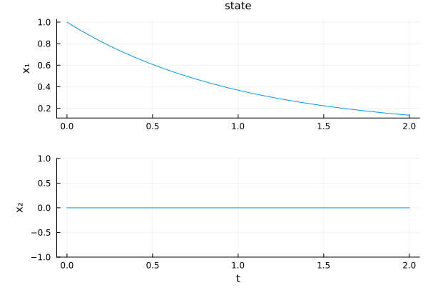
hsol = hmpf((0.0, 2.0), x0, p0)
plot(hsol)  # state and costate, across both phases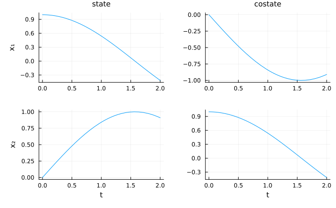
Different dynamics — kink at the switching time
When the two phases use different vector fields, the slope changes abruptly at the switching time. The trajectory is continuous but not differentiable:
# phase 1: f(x) = -x   |   phase 2: f(x) = -2x
sol_het = mpf_het((0.0, 2.0), x0)
plot(sol_het)   # kink visible at t = 1.0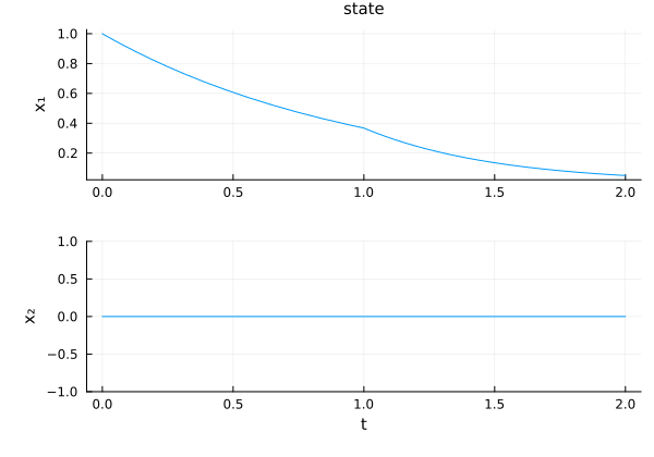
State jump — discontinuity in state
A non-zero additive jump x ← x + jump_x produces a visible discontinuity in the state trajectory:
# jump_x = [0.5, 0.0] defined above
sol_jump = mpf_jump((0.0, 2.0), x0)
plot(sol_jump)   # state jumps by [0.5, 0.0] at t = 1.0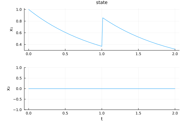
Hamiltonian flow — costate jump
For Hamiltonian flows, hflow1 * (t, jump_p, hflow2) adds an additive vector to the costate (p ← p + jump_p). The state remains continuous:
jump_p = [0.0, 0.5]
hmpf_jp = hflow1 * (1.0, jump_p, hflow2)
hsol_jp = hmpf_jp((0.0, 2.0), x0, p0)
plot(hsol_jp)   # costate jumps by [0.0, 0.5] at t = 1.0, state unchanged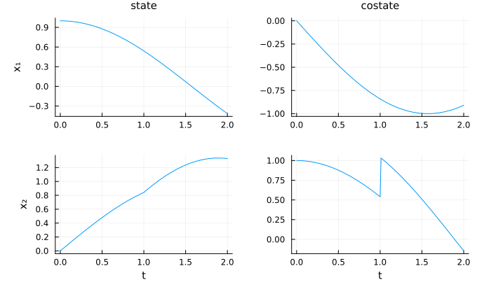
Hamiltonian flow — simultaneous state and costate jump
hflow1 * (t, jump_x, jump_p, hflow2) jumps both components at once (x ← x + jump_x, p ← p + jump_p):
jump_xx, jump_pp = [0.1, 0.0], [0.0, 0.5]
hmpf_jxp = hflow1 * (1.0, jump_xx, jump_pp, hflow2)
hsol_jxp = hmpf_jxp((0.0, 2.0), x0, p0)
plot(hsol_jxp)   # both state and costate jump at t = 1.0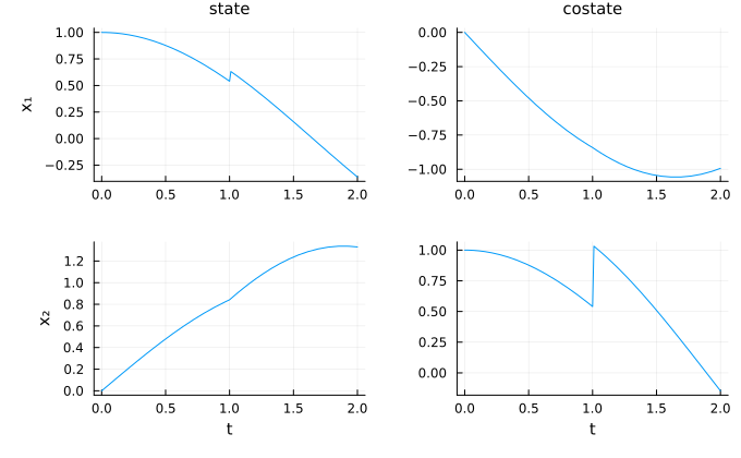
State function jump
A callable f(x) transforms the state at the switching time:
mpf_fn = flow1 * (1.0, x -> 2.0 .* x, flow2)
sol_fn = mpf_fn((0.0, 2.0), x0)
plot(sol_fn)   # state doubled at t = 1.0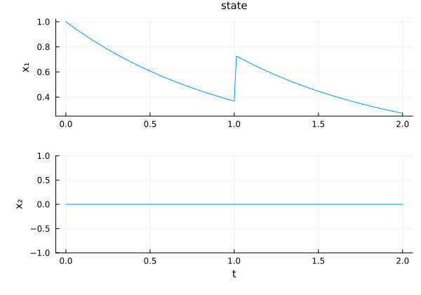
Hamiltonian function jump — full transformation
A callable f(x, p) transforms both components simultaneously:
hmpf_fn = hflow1 * (
    1.0, (x, p) -> (2.0 .* x, p .+ 0.5), hflow2
)
hsol_fn = hmpf_fn((0.0, 2.0), x0, p0)
plot(hsol_fn)   # state doubled, costate shifted at t = 1.0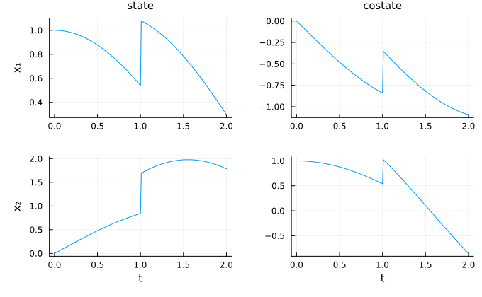
Hamiltonian state-only jump
Using nothing for the costate component leaves it unchanged:
hmpf_sx = hflow1 * (1.0, [0.1, 0.0], nothing, hflow2)
hsol_sx = hmpf_sx((0.0, 2.0), x0, p0)
plot(hsol_sx)   # state jumps, costate continuous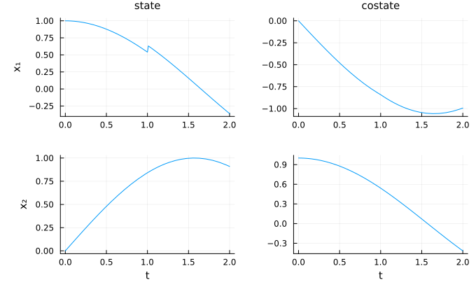
Design notes
Concatenation is an associative binary operation on flows:
(f1 * (t, f2)) * (s, f3).Phases may have different system and integrator types (
S,I): each phase can wrap a distinct function and use its own solver. Theflowsfield is a heterogeneous tuple, so the compiler specializes the integration loop per phase combination. The required uniformity across phases isTD,VD, and the dynamics family (state vs Hamiltonian), enforced at construction time.The trajectory integration merges phase results via
Integrators.merge, which concatenates the time grids and result vectors.
See also
CTFlows.MultiPhase.MultiPhaseStateFlow,CTFlows.MultiPhase.MultiPhaseHamiltonianFlow,CTFlows.MultiPhase.AnyMultiPhaseFlow— multi-phase flow types.CTFlows.MultiPhase.n_phases,CTFlows.MultiPhase.get_flow,CTFlows.MultiPhase.get_switching_time,CTFlows.MultiPhase.get_jump— phase accessors.CTFlows.MultiPhase.get_flows,CTFlows.MultiPhase.get_switching_times,CTFlows.MultiPhase.get_jumps— bulk accessors.