SciML flows
The CTFlowsSciMLFlows extension (activated by loading SciMLBase, e.g. through any OrdinaryDiffEq solver package) lets Flows.Flow consume SciML objects directly:
Flow(f::SciMLBase.AbstractODEFunction)— wraps the function in aSciMLFunctionSystemand runs the standard pipeline, producing aStateFlow.Flow(prob::SciMLBase.AbstractODEProblem)— wraps the fully-assembled problem in aSciMLProblemFlow, bypassing the system-building pipeline (the problem already carriesu0,tspanandp).
This is the bridge for users who already have SciML code and want the CTFlows call interface (point/trajectory styles, configs, multi-phase concatenation).
From an ODEFunction
f = SciMLBase.ODEFunction((du, u, p, t) -> du .= -p .* u)
flow = Flows.Flow(f; reltol=1e-10)
Flow
├─ system: SciMLFunctionSystem
│ └─ wraps: ODEFunction: non-autonomous, variable, in-place
└─ integrator: SciML{CPU} (instance, id=:sciml)
├─ internalnorm = real_norm [default]
├─ alg = Tsit5 [default]
├─ reltol = 1.0e-10 [user]
├─ save_everystep = auto [default]
├─ abstol = 1.0e-8 [default]
├─ save_start = auto [default]
└─ dense = auto [default]
Tip: use describe(SciML{CPU}) to see all available options.The resulting flow behaves like any StateFlow. SciML functions receive their parameter through p, which CTFlows maps to the variable keyword:
julia> xf = flow(0.0, [1.0], 1.0; variable=2.0)   # ≈ exp(-2)
0.1353352833736127
Trajectory calls work the same way, returning a VectorFieldTrajectory — plot it directly once Plots is loaded:
sol = flow((0.0, 1.0), [1.0]; variable=2.0)VectorFieldTrajectory
├─ result: SciMLIntegrationResult
├─ tspan: (0.0, 1.0)
├─ time points: 28
├─ final state: 0.1353352833736127
└─ variable: 2.0plot(sol)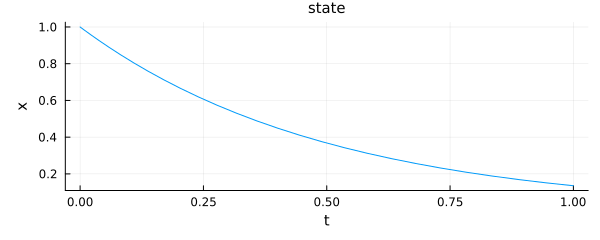
Traits of SciML-backed flows
A SciML function has the uniform (du, u, p, t) signature, so the wrapped flow is always NonAutonomous / NonFixed: pass the parameter via variable at call time.
From an ODEProblem
A problem already bundles the dynamics, initial condition, time span, and parameter. Flows.Flow wraps it in a SciMLProblemFlow:
prob = SciMLBase.ODEProblem((du, u, p, t) -> du .= -p .* u, [1.0], (0.0, 1.0), 2.0)
pflow = Flows.Flow(prob; reltol=1e-10)
SciMLProblemFlow
├─ tspan: (0.0, 1.0)
├─ u0: [1.0]
└─ integrator: SciML{CPU} (instance, id=:sciml)
├─ internalnorm = real_norm [default]
├─ alg = Tsit5 [default]
├─ reltol = 1.0e-10 [user]
├─ save_everystep = auto [default]
├─ abstol = 1.0e-8 [default]
├─ save_start = auto [default]
└─ dense = auto [default]
Tip: use describe(SciML{CPU}) to see all available options.SciMLProblemFlow supports three call modes:
julia> result = pflow();                       # no-arg: solve the problem as-is

julia> Integrators.final_state(result)
1-element Vector{Float64}:
 0.1353352833736127

julia> xf = pflow(0.5, [2.0], 2.0; variable=3.0)   # point call: remake, final state
1-element Vector{Float64}:
 0.022217993247402586

julia> result = pflow((0.5, 2.0), [2.0]; variable=3.0);  # trajectory call: remake, full result

julia> Integrators.times(result)[end]
2.0
Point and trajectory calls go through SciMLBase.remake, replacing u0, tspan and (when variable is given) p before solving. The no-arg and trajectory calls return an AbstractIntegrationResult — use Integrators.times, Integrators.evaluate_at and Integrators.final_state to inspect it (see Trajectories).
See also
CTFlowsSciMLFlows.SciMLProblemFlow,CTFlowsSciMLFlows.SciMLFunctionSystem— the extension types.CTFlows.Flows.Flow— the constructor family.CTSolvers.Integrators.times,CTSolvers.Integrators.evaluate_at,CTSolvers.Integrators.final_state— result accessors.Integrating — call styles and integrator options.