Control laws

When the dynamical system depends on a control , the flow cannot be integrated directly: the control must be eliminated by a control law that expresses as a function of the available state variables. CTFlows supports three kinds of control laws, each leading to a different flow type.

Control law types

All control laws live in CTBase.Data and are constructed by wrapping a function:

Law	Constructor	Feedback signature	Available state
`OpenLoop`	`Data.OpenLoop(u)`	`u(t, v)`	none (time only)
`ClosedLoop`	`Data.ClosedLoop(u)`	`u(t, x, v)`	state
`DynClosedLoop`	`Data.DynClosedLoop(u)`	`u(t, x, p, v)`	state + costate

The trait CTBase.Traits.feedback distinguishes the three and drives dispatch in Flow constructors.

Two flow paths

Law type	Flow type	Dynamics	Trajectory result
`DynClosedLoop`	`HamiltonianFlow` / `OptimalControlFlow`	Hamiltonian (state + costate)	`HamiltonianVectorFieldTrajectory` / `CTModels.Solution`
`OpenLoop` / `ClosedLoop`	`ControlledFlow` (state flow)	state only	`StateFlowTrajectory`

A DynClosedLoop law needs the costate to evaluate the feedback, so it produces a Hamiltonian flow. An OpenLoop or ClosedLoop law does not need , so the control is eliminated upfront and the system is integrated as a state flow.

`Flow(h̃, law)` — pseudo-Hamiltonian + DynClosedLoop

A Data.PseudoHamiltonian wraps the function . Combined with a DynClosedLoop law , the control is substituted to form the closed-loop Hamiltonian .

The hamiltonian_type keyword controls how AD is applied:

:total (default): compose with the law into a Data.ComposedHamiltonian and differentiate through the law (total derivative).
:partial: build a CTFlows.Systems.PseudoHamiltonianSystem that takes partial derivatives of at the fixed feedback value . This coincides with :total only where the feedback is stationary ().

julia

# Pseudo-Hamiltonian: H̃(x, p, u) = p * u - 0.5 * u^2  (maximised at u = p)
h̃ = Data.PseudoHamiltonian((x, p, u) -> p * u - 0.5 * u^2)
law = Data.DynClosedLoop((x, p) -> p)  # u = p

# Total mode (default): AD through the law
f_total = Flows.Flow(h̃, law; reltol=1e-10)

# Partial mode: AD at fixed u
f_partial = Flows.Flow(h̃, law; hamiltonian_type=:partial, reltol=1e-10)

Flow
├─ system: PseudoHamiltonianSystem
│          ├─ time_dependence: Autonomous
│          ├─ variable_dependence: Fixed
│          ├─ PseudoHamiltonian: autonomous, fixed (no variable)
│          │    natural call: h̃(x, p, u)
│          │    uniform call: h̃(t, x, p, u, v)
│          ├─ ControlLaw: dyn-closed-loop, autonomous, fixed (no variable)
│          │    natural call: u(x, p)
│          │    uniform call: u(t, x, p, v)
│          └─ backend: DifferentiationInterface(ad_backend=AutoForwardDiff())
└─ integrator: SciML (reltol = 1.0e-10)

Because the flow was built from a pseudo-Hamiltonian and a law, it exposes them (and the resulting closed-loop Hamiltonian) through the Systems getters — these throw an IncorrectArgument on a plain HamiltonianFlow that carries no law:

julia

Systems.pseudo_hamiltonian(f_total)   # H̃(t, x, p, u, v)

PseudoHamiltonian: autonomous, fixed (no variable)
  natural call: h̃(x, p, u)
  uniform call: h̃(t, x, p, u, v)

julia

Systems.control_law(f_total)          # the DynClosedLoop feedback u(t, x, p, v)

ControlLaw: dyn-closed-loop, autonomous, fixed (no variable)
  natural call: u(x, p)
  uniform call: u(t, x, p, v)

julia

Systems.hamiltonian(f_total)          # closed-loop H(t, x, p, v) = H̃(…, u(…), …)

ComposedHamiltonian: autonomous, fixed (no variable)
  natural call: h(x, p)
  uniform call: h(t, x, p, v)

OpenLoop/ClosedLoop rejected

A PseudoHamiltonian depends on the costate , which OpenLoop and ClosedLoop laws do not provide. Passing one raises a PreconditionError.

`Flow(fc, law)` — controlled vector field + OpenLoop/ClosedLoop

A Data.ControlledVectorField wraps . Combined with an OpenLoop or ClosedLoop law, the control is eliminated via a Data.ComposedVectorField , and the result is integrated as a state flow. The resulting ControlledFlow carries no OCP, so trajectory calls return a StateFlowTrajectory without an objective.

julia

# Controlled dynamics: ẋ = -x + u
fc = Data.ControlledVectorField((x, u) -> -x + u)
law = Data.ClosedLoop(x -> -x)  # feedback u = -x

f = Flows.Flow(fc, law; reltol=1e-8)

ControlledFlow
├─ system: VectorFieldSystem
│          ├─ wraps: VectorField: autonomous, fixed (no variable), out-of-place
│          └─ rhs: IPVFOoPRHS (out-of-place VF → in-place interface)
└─ integrator: SciML (reltol = 1.0e-8)

DynClosedLoop rejected

A DynClosedLoop law needs the costate , which a state flow does not have. Use Flow(h̃, law) or Flow(ocp, law) instead.

`Flow(ocp, law)` — OCP + control law

For an OCP with control, pass a control law to Flow(ocp, law). The constructor dispatches on the law's feedback trait:

DynClosedLoop → `OptimalControlFlow`

The OCP's dynamics and cost supply the pseudo-Hamiltonian . The law closes the loop and the resulting flow is an OptimalControlFlow — point calls behave like a HamiltonianFlow, trajectory calls return a CTModels.Solutions.Solution with the control reconstructed from the law.

The hamiltonian_type keyword (:total default, :partial) works as in Flow(h̃, law).

julia

# OCP: ẋ = -x + u, min ∫ 0.5*u^2 dt  (autonomous, fixed, 1-D — scalar convention)
pre = CTModels.Building.PreModel()
CTModels.Building.time_dependence!(pre; autonomous=true)
CTModels.Building.time!(pre; t0=0.0, tf=1.0)
CTModels.Building.state!(pre, 1)
CTModels.Building.control!(pre, 1)
CTModels.Building.dynamics!(pre, (r, t, x, u, v) -> (r[1] = -x + u; nothing))
CTModels.Building.objective!(pre, :min; lagrange=(t, x, u, v) -> 0.5 * u^2)
ocp = CTModels.Building.build(pre)

julia

# DynClosedLoop law: u(x, p) = p  (from PMP, maximises H̃ = p*(-x+u) - 0.5*u^2)
law = Data.DynClosedLoop((x, p) -> p)
f_ocp = Flows.Flow(ocp, law; reltol=1e-10)

OptimalControlFlow
├─ system: HamiltonianSystem
│          ├─ time_dependence: Autonomous
│          ├─ variable_dependence: Fixed
│          ├─ ComposedHamiltonian: autonomous, fixed (no variable)
│          │    natural call: h(x, p)
│          │    uniform call: h(t, x, p, v)
│          └─ backend: DifferentiationInterface(ad_backend=AutoForwardDiff())
└─ integrator: SciML (reltol = 1.0e-10)

Point evaluation returns the final state–costate pair:

julia

julia> x0, p0 = 1.0, 0.5;

julia> xf, pf = f_ocp(0.0, x0, p0, 1.0);

julia> xf
0.9554800380788495

julia> pf
1.3591409143138347

Trajectory evaluation returns a CTModels.Solution, with the control reconstructed from the law:

julia

sol = f_ocp((0.0, 1.0), x0, p0)
CTModels.Components.objective(sol)

0.39931600619415

Once Plots is loaded it draws directly — state, costate, and the reconstructed control :

julia

plot(sol)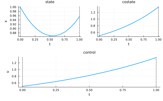

OpenLoop / ClosedLoop → `ControlledFlow`

The OCP's controlled dynamics are extracted as a ControlledVectorField, the law eliminates the control, and the result is a ControlledFlow — a state flow. Point calls return the final state (no costate); trajectory calls return a StateFlowTrajectory with state, reconstructed control, and objective (Mayer + Lagrange).

julia

# OpenLoop law: u() = 1 (constant, autonomous ⇒ no time argument)
law_ol = Data.OpenLoop(() -> 1.0)
f_cflow = Flows.Flow(ocp, law_ol; reltol=1e-8)

ControlledFlow
├─ system: VectorFieldSystem
│          ├─ wraps: VectorField: autonomous, fixed (no variable), out-of-place
│          └─ rhs: IPVFOoPRHS (out-of-place VF → in-place interface)
└─ integrator: SciML (reltol = 1.0e-8)

julia

julia> xf_c = f_cflow(0.0, 1.0, 1.0)
1.0

julia

sol_c = f_cflow((0.0, 1.0), 1.0)
Trajectories.objective(sol_c)   # ≈ 0.5 * 1^2 * 1 = 0.5

0.4999999999999999

Convenience: `Flow(ocp, u::Function)`

A plain function u is wrapped in a DynClosedLoop law automatically, with time/variable dependence inferred from the OCP:

julia

f_conv = Flows.Flow(ocp, (x, p) -> p; reltol=1e-10)  # autonomous, fixed → auto DynClosedLoop

OptimalControlFlow
├─ system: HamiltonianSystem
│          ├─ time_dependence: Autonomous
│          ├─ variable_dependence: Fixed
│          ├─ ComposedHamiltonian: autonomous, fixed (no variable)
│          │    natural call: h(x, p)
│          │    uniform call: h(t, x, p, v)
│          └─ backend: DifferentiationInterface(ad_backend=AutoForwardDiff())
└─ integrator: SciML (reltol = 1.0e-10)

The function u must have the natural arity matching the OCP's traits: (x, p), (t, x, p), (x, p, v), or (t, x, p, v). To use a law whose traits differ from the OCP's, construct the DynClosedLoop explicitly.

`ControlledFlow` type

A ControlledFlow wraps:

an inner state Flow integrating the closed-loop dynamics ,
an optional OCP (for the objective),
the control law (for reconstructing ).

It is a subtype of AbstractFlow with StateDynamics. Point evaluation returns the final state (no costate); trajectory evaluation returns a StateFlowTrajectory.

`StateFlowTrajectory`

A StateFlowTrajectory is the result of a trajectory call on a ControlledFlow. It provides:

Accessor	Returns	Notes
`state(sol)`	callable `x(t)`	state trajectory (scalar coercion for 1-D state)
`control(sol)`	callable `u(t)`	reconstructed from the law: `u(t) = law(t, x(t), v)`
`objective(sol)`	`Real` or `nothing`	Mayer + Lagrange (only when built from an OCP)
`time_grid(sol)`	vector of time points
`costate(sol)`	—	errors: a state flow has no costate

julia

x_c = Trajectories.state(sol_c)
u_c = Trajectories.control(sol_c)
x_c(0.5), u_c(0.5)

(1.0, 1.0)

A StateFlowTrajectory plots its state and reconstructed control together (its default panels are (:state, :control)):

julia

plot(sol_c)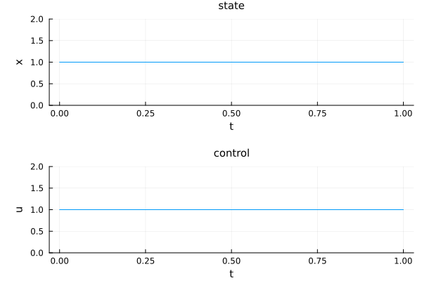

Summary table

Constructor	Law type	Resulting flow	Trajectory type
`Flow(h̃, law)`	`DynClosedLoop`	`HamiltonianFlow`	`HamiltonianVectorFieldTrajectory`
`Flow(fc, law)`	`OpenLoop` / `ClosedLoop`	`ControlledFlow`	`StateFlowTrajectory` (no objective)
`Flow(ocp, law)`	`DynClosedLoop`	`OptimalControlFlow`	`CTModels.Solution`
`Flow(ocp, law)`	`OpenLoop` / `ClosedLoop`	`ControlledFlow`	`StateFlowTrajectory` (with objective)
`Flow(ocp, u::Function)`	`DynClosedLoop` (auto)	`OptimalControlFlow`	`CTModels.Solution`

Control laws ​

Control law types ​

Two flow paths ​

Flow(h̃, law) — pseudo-Hamiltonian + DynClosedLoop ​

Flow(fc, law) — controlled vector field + OpenLoop/ClosedLoop ​

Flow(ocp, law) — OCP + control law ​

DynClosedLoop → OptimalControlFlow ​

OpenLoop / ClosedLoop → ControlledFlow ​

Convenience: Flow(ocp, u::Function) ​

ControlledFlow type ​

StateFlowTrajectory ​

Summary table ​

See also ​

Control laws

Control law types

Two flow paths

`Flow(h̃, law)` — pseudo-Hamiltonian + DynClosedLoop

`Flow(fc, law)` — controlled vector field + OpenLoop/ClosedLoop

`Flow(ocp, law)` — OCP + control law

DynClosedLoop → `OptimalControlFlow`

OpenLoop / ClosedLoop → `ControlledFlow`

Convenience: `Flow(ocp, u::Function)`

`ControlledFlow` type

`StateFlowTrajectory`

Summary table

See also