Trajectories
A trajectory integration returns a solution object that wraps the raw ODE result and exposes semantic accessors. The CTFlows.Trajectories submodule provides these wrappers.
Solution types
A trajectory call returns one of three CTFlows containers, depending on the flow:
| Type | Produced by | Content |
|---|---|---|
VectorFieldTrajectory | StateFlow trajectory call | state trajectory |
HamiltonianVectorFieldTrajectory | HamiltonianFlow trajectory call | state + costate trajectories |
StateFlowTrajectory | ControlledFlow trajectory call | state + reconstructed control (+ objective when from an OCP) |
A fourth result appears one level up: a trajectory call on an OptimalControlFlow (a control-free Flow(ocp), or Flow(ocp, law) with a DynClosedLoop law) returns a CTModels.Solutions.Solution rather than a CTFlows container — see Optimal control. All four share the same accessor vocabulary (state, costate, control, objective) and the same plot / plot! entry point (Plots or Makie backend — see Plotting below).
VectorFieldTrajectory
sol # produced by flow((t0, tf), x0)VectorFieldTrajectory
├─ result: SciMLIntegrationResult
├─ tspan: (0.0, 1.0)
├─ time points: 16
└─ final state: [0.36787944127643135, 0.0]Accessors
| Accessor | Returns | Notes |
|---|---|---|
state(sol) | callable x(t) | returns sol itself, which is callable |
time_grid(sol) | vector of time points | alias for times(sol) |
final_state(sol) | Vector | the final state x(tf) |
status(sol) / successful(sol) | retcode / Bool | solver outcome (see Solver status) |
ts = Trajectories.time_grid(sol)   # vector of time points
ts[1], ts[end]
(0.0, 1.0)x = Trajectories.state(sol) # callable: x(t) → state at time t
x(0.0) # initial state (exact)2-element Vector{Float64}:
1.0
0.0x(0.5) # interpolated at t = 0.52-element Vector{Float64}:
0.6065306592843307
0.0x.(ts) # broadcast over the time grid16-element Vector{Vector{Float64}}:
[1.0, 0.0]
[0.9877640316387758, 0.0]
[0.9586392120306756, 0.0]
[0.9219104181991034, 0.0]
[0.8795807933369617, 0.0]
[0.8322170230625516, 0.0]
[0.7816374670004691, 0.0]
[0.7290594161179201, 0.0]
[0.6758982310332805, 0.0]
[0.6231970367115284, 0.0]
[0.5718586020913711, 0.0]
[0.52252001337596, 0.0]
[0.47564070023807803, 0.0]
[0.43150217019049936, 0.0]
[0.3902590168711898, 0.0]
[0.36787944127643146, 0.0]state(sol) returns sol itself, which is callable. The two forms state(sol)(t) and sol(t) are equivalent. time_grid is an alias for times.
Point integration vs trajectory
Point integration (flow(t0, x0, tf)) returns the final state directly as a Vector, not a solution object:
xf = flow(0.0, x0, 1.0)   # Vector, not VectorFieldTrajectory
typeof(xf)
Vector{Float64} (alias for Array{Float64, 1})Use trajectory integration (flow((t0, tf), x0)) when you need the full history.
HamiltonianVectorFieldTrajectory
hsol # produced by hflow((t0, tf), x0, p0)HamiltonianVectorFieldTrajectory
├─ result: SciMLIntegrationResult
├─ tspan: (0.0, 1.0)
├─ time points: 18
├─ final state: [0.540302305784261, 0.8414709847533872]
└─ final costate: [-0.8414709847533872, 0.540302305784261]Accessors
| Accessor | Returns | Notes |
|---|---|---|
state(sol) | callable x(t) | state trajectory |
costate(sol) | callable p(t) | costate trajectory |
time_grid(sol) | vector of time points | alias for times(sol) |
final_state(sol) | (xf, pf) | final state–costate pair |
status(sol) / successful(sol) | retcode / Bool | solver outcome |
ts_h = Trajectories.time_grid(hsol)18-element Vector{Float64}:
0.0
0.010717734625362933
0.03678924587914857
0.07082975288098367
0.11171621300174836
0.15977761725931772
0.21406631262527503
0.2741409966210073
0.3391635630607941
0.40850604198933127
0.48147597812035614
0.5575059231266913
0.6360680321223101
0.7167220825435473
0.7990884851440955
0.882851471167152
0.9677468775678141
1.0x_h = Trajectories.state(hsol) # state trajectory: x(t)
p_h = Trajectories.costate(hsol) # costate trajectory: p(t)
x_h(0.0), p_h(0.0)([1.0, 0.0], [0.0, 1.0])x_h(0.5), p_h(0.5)([0.8775825617654902, 0.479425538879898], [-0.479425538879898, 0.8775825617654902])StateFlowTrajectory
A StateFlowTrajectory is produced by a trajectory call on a ControlledFlow (see Control laws). It wraps a state trajectory with a reconstructed control and an optional objective.
Accessors
| Accessor | Returns | Notes |
|---|---|---|
state(sol) | callable x(t) | state trajectory (scalar coercion for 1-D) |
control(sol) | callable u(t) | reconstructed from the law: u(t) = law(t, x(t), v) |
objective(sol) | Real | Mayer + Lagrange — errors unless built from an OCP |
time_grid(sol) | vector of time points | alias for times(sol) |
final_state(sol) | Vector | the final state x(tf) |
status(sol) / successful(sol) | retcode / Bool | solver outcome |
costate(sol) | — | errors: a state flow has no costate |
The cflow in this page's setup is a ControlledFlow built from Flow(fc, law) (no OCP), so its trajectory csol carries a state and a reconstructed control:
x_c = Trajectories.state(csol)     # x(t)
u_c = Trajectories.control(csol)   # u(t) = law(t, x(t), v)
x_c(0.5), u_c(0.5)
(0.36787944126257494, -0.36787944126257494)objective(csol) and costate(csol) raise a PreconditionError here: this flow has no OCP (so no cost) and is a state flow (so no costate). Build from an OCP — Flow(ocp, law) — to get the objective; see Control laws.
Solver status and final state
Every trajectory forwards the integrator's outcome and its final value from the underlying result — the same accessors work on all three container types:
Integrators.status(sol), Integrators.successful(sol)(:Success, true)Integrators.final_state(sol) # xf — a state flow returns the state2-element Vector{Float64}:
0.36787944127643135
0.0Integrators.final_state(hsol) # (xf, pf) — a Hamiltonian flow returns the pair([0.540302305784261, 0.8414709847533872], [-0.8414709847533872, 0.540302305784261])status returns the integrator's return code and successful a Bool. A point call raises a SolverFailure on a non-success code unless unsafe=true; a trajectory call always returns, so inspect successful(sol) to check convergence (see Integrating).
Plotting
Trajectory plotting is split into a backend-free case layer and a backend:
CTFlows.TrajectoryPlots(insrc/) turns a trajectory plus adescriptioninto aCTBase.Plotting.Figure— vocabulary (:state,:costate,:control), panels, layout. It has no plotting dependency. The single entry point isCTFlows.TrajectoryPlots.build_figure, which also owns the user-facing defaults.a weak-dependency extension wires a rendering backend to
plot/plot!on the trajectory types:
| Extension | Trigger | plot(traj) returns | Renders via |
|---|---|---|---|
CTFlowsPlots | using Plots | Plots.Plot | CTBase.Plotting.PlotsBackend |
CTFlowsMakie | using CairoMakie / GLMakie (any Makie) | Makie.Figure | CTBase.Plotting.MakieBackend |
Both extensions call build_figure and hand the figure to CTBase.Plotting.render(<backend>, fig); they expose the same description and keyword surface. The Makie backend is at feature parity with the Plots backend (see CTModels#408 / CTBase#540). Until a backend extension is loaded, plot on a trajectory throws a CTBase.Exceptions.ExtensionError.
When only one backend is loaded, call plot unqualified; when both are loaded (as in this build), qualify — Plots.plot(traj) vs Makie.plot(traj).
Plots.plot(sol) # each state component — Plots backend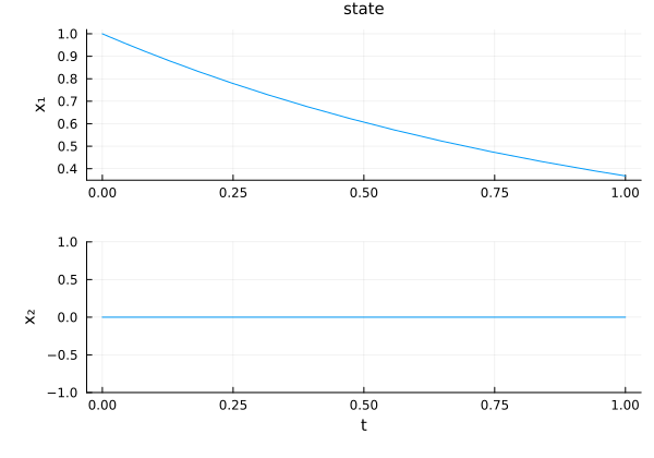
Makie.plot(hsol) # state and costate components — Makie backend, a Makie.Figure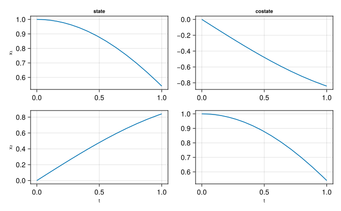
Plot options
Each container draws a default set of panels: VectorFieldTrajectory → state, HamiltonianVectorFieldTrajectory → state + costate, StateFlowTrajectory → state + control. Pass description symbols (:state, :costate, :control) to select panels, and keywords to tune the layout — identical on both backends:
| Keyword | Values | Effect |
|---|---|---|
layout | :split (default) / :group | one subplot per component, or all in one cell |
control | :components (default) / :norm / :all | each control, its norm, or both |
time | :default (default) / :normalize | real time, or rescaled to |
state_style, costate_style, control_style | NamedTuple / :none | per-group backend attributes, or hide the group |
size | (w, h) | figure size in pixels |
Any further keyword is forwarded to the backend (see CTFlows.TrajectoryPlots.split_plot_kwargs).
Plots.plot(hsol, :state; layout=:group, time=:normalize) # only the state, grouped, [0,1] time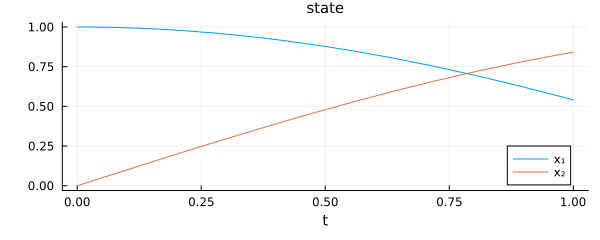
Makie.plot(hsol, :state; layout=:group, time=:normalize) # same call, Makie backend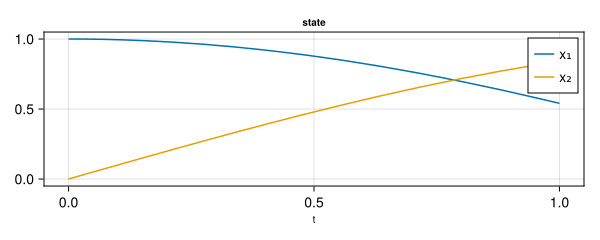
plot! overlays a second trajectory onto an existing figure, on either backend:
f = Makie.plot(hsol)
Makie.plot!(f, hsol; state_style=(linestyle=:dash,))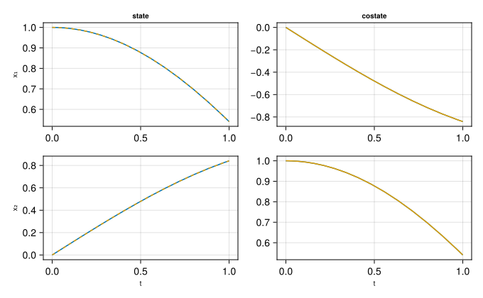
Low-level: integration result
Under the hood, solution objects wrap an AbstractIntegrationResult which exposes:
Integrators.times(result)— the time gridIntegrators.evaluate_at(result, t)— interpolated value attIntegrators.final_state(result)— the final value
These are used internally by the solution wrappers and normally not called directly.
See also
CTFlows.Trajectories.VectorFieldTrajectory,CTFlows.Trajectories.HamiltonianVectorFieldTrajectory,CTFlows.Trajectories.StateFlowTrajectory— solution container types.CTFlows.Trajectories.state,CTFlows.Trajectories.costate,CTFlows.Trajectories.control,CTFlows.Trajectories.objective— trajectory accessors.CTFlows.Trajectories.time_grid,CTSolvers.Integrators.times— time grid accessors.CTSolvers.Integrators.final_state,CTSolvers.Integrators.status,CTSolvers.Integrators.successful,CTSolvers.Integrators.evaluate_at— result / status accessors.