Optimal control
Flows.Flow accepts an optimal control problem — a CTModels.Models.Model — and builds the flow of the associated Hamiltonian system directly from the problem structure. The result is an OptimalControlFlow: point calls behave like a HamiltonianFlow, while trajectory calls return a full CTModels.Solutions.Solution.
Control-free problems
The no-law constructor Flow(ocp) dispatches on the problem's CTBase.Traits.ControlDependence trait:
Control-free (
ControlFree): the pseudo-Hamiltonian reduces to:min,:max). The state equationWith control (
WithControl): aPreconditionErroris thrown. UseFlow(ocp, law)to pass a control law — see Control laws.
Building the flow
Define a control-free problem with the CTModels building API (the exponential dynamics
λ = 2.0

pre = CTModels.Building.PreModel()
CTModels.Building.time_dependence!(pre; autonomous=true)
CTModels.Building.time!(pre; t0=0.0, tf=1.0)
CTModels.Building.state!(pre, 1)
CTModels.Building.dynamics!(pre, (r, t, x, u, v) -> (r[1] = λ * x[1]; nothing))
CTModels.Building.objective!(pre, :min; mayer=(x0, xf, v) -> xf[1])
ocp = CTModels.Building.build(pre)
Then hand it to Flows.Flow:
f = Flows.Flow(ocp; reltol=1e-10, abstol=1e-10)OptimalControlFlow
├─ system: HamiltonianSystem
│ ├─ time_dependence: Autonomous
│ ├─ variable_dependence: Fixed
│ ├─ Hamiltonian: autonomous, fixed (no variable)
│ │ natural call: h(x, p)
│ │ uniform call: h(t, x, p, v)
│ └─ backend: DifferentiationInterface{CPU}(ad_backend=AutoForwardDiff)
└─ integrator: SciML{CPU} (instance, id=:sciml)
├─ internalnorm = real_norm [default]
├─ alg = Tsit5 [default]
├─ reltol = 1.0e-10 [user]
├─ save_everystep = auto [default]
├─ abstol = 1.0e-10 [user]
├─ save_start = auto [default]
└─ dense = auto [default]
Tip: use describe(SciML{CPU}) to see all available options.Keyword options are routed exactly as for Flow(h::Data.AbstractHamiltonian): integrator options (reltol, abstol, alg, …) go to the SciML strategy, AD options (ad_backend) to the DifferentiationInterface strategy.
Point calls — Hamiltonian semantics
Point evaluation delegates to the inner HamiltonianFlow and returns the final state–costate pair. For
julia> x0, p0 = 1.0, 1.0;

julia> xf, pf = f(0.0, x0, p0, 1.0);

julia> xf   # ≈ exp(λ)
7.389056098963722

julia> pf   # ≈ exp(-λ)
0.1353352832375321
The variable, variable_costate and unsafe keywords work as for any Hamiltonian flow — see Integrating.
Free times
Flow(ocp) builds an OptimalControlFlow around an inner HamiltonianFlow, so the same free-time shooting technique described in Integrating § Variable costate applies directly: a free variable, and t1 in f(t0, x0, p0, t1; variable=v) is the evaluation time — independent of v, even when v represents the free endpoint being shot on.
Because the augmented costate is initialised at H = Systems.hamiltonian(f) — with an opposite sign convention at each end:
See test/suite/flows/test_variable_costate_free_time.jl for worked examples that exercise this
Trajectory calls — a CTModels.Solution
A trajectory call integrates the Hamiltonian system and assembles a complete CTModels.Solutions.Solution: state and costate interpolants, an empty control (the problem is control-free), and the objective value (Mayer, Lagrange, or Bolza — a Lagrange cost is integrated with the same integrator).
sol = f((0.0, 1.0), x0, p0)Solution ✓ successful
│ Objective : 7.389056098963722
│ Status : Success
└─ Message : Solution computed by CTFlows OCP flowUse the standard CTModels accessors on the result:
julia> CTModels.Components.objective(sol)    # ≈ exp(λ)
7.389056098963722

julia> CTModels.Components.state(sol)(0.5)   # x(0.5) ≈ exp(λ/2)
2.7182818284893293

julia> CTModels.Components.costate(sol)(0.5) # p(0.5) ≈ exp(-λ/2)
0.3678794411684144
Because the result is a CTModels.Solution, it plots directly once Plots is loaded — state and costate on a shared time axis (the control panel is empty, the problem being control-free):
plot(sol)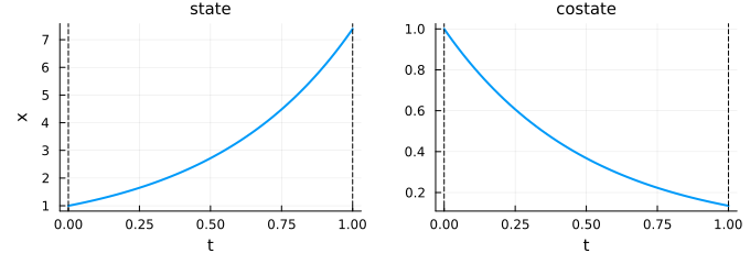
Basic flow — no costate (direct shooting)
For a control-free OCP, Flow(ocp) also exposes a state-only call, with no costate — the direct-shooting use case (#230). Same f object, dispatched on arity (3 positional arguments instead of 4):
julia> xf_basic = f(0.0, x0, 1.0)
7.389056098956882

julia> xf_basic ≈ xf
true
A trajectory call returns a StateFlowTrajectory with law = nothing: state and objective are available, but the flow carries neither a control nor a costate, so control/costate raise a PreconditionError:
sol_basic = f((0.0, 1.0), x0)StateFlowTrajectory
├─ tspan: (0.0, 1.0)
├─ time points: 62
├─ final state: 7.389056098956882
└─ objective: 7.389056098956881julia> using CTFlows: Trajectories
julia> Trajectories.state(sol_basic)(0.5)
2.7182818284646686
julia> Trajectories.objective(sol_basic) # ≈ exp(λ)
7.389056098956881Flow(ocp, law) has no such basic call when law is DynClosedLoop: its dynamics depend on the costate p(t), so f(t0, x0, tf) raises a PreconditionError suggesting f(t0, x0, p0, tf) instead. For an OpenLoop/ClosedLoop law, the state-only equivalent already exists as the ControlledFlow returned by Flow(ocp, law) — see Control laws.
Inspecting the wrapper
OptimalControlFlow is a thin AbstractFlow wrapper around the inner HamiltonianFlow; it exists solely so the trajectory call can rebuild a CTModels.Solution from the problem:
julia> Flows.system(f) isa CTFlows.Systems.HamiltonianSystem
true

julia> Traits.time_dependence(f)
CTBase.Traits.Autonomous
See also
CTFlows.Flows.OptimalControlFlow— the wrapper type.CTFlows.Flows.Flow— the constructor family, includingFlow(ocp).CTModels.Solutions.Solution,CTModels.Components.objective— the trajectory-call result and its accessors.Control laws —
Flow(ocp, law)for with-control problems.Constrained flows —
constraint/multiplierpath-constraint terms.Building a flow — AD-backed Hamiltonian flows.