Basic example (functional version)

Let us consider a wagon moving along a rail, whom acceleration can be controlled by a force $u$. We denote by $x = (x_1, x_2)$ the state of the wagon, that is its position $x_1$ and its velocity $x_2$.

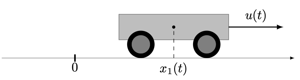
We assume that the mass is constant and unitary and that there is no friction. The dynamics we consider is given by

\[ \dot x_1(t) = x_2(t), \quad \dot x_2(t) = u(t), \quad u(t) \in \R,\]

which is simply the double integrator system. Les us consider a transfer starting at time $t_0 = 0$ and ending at time $t_f = 1$, for which we want to minimise the transfer energy

\[ \frac{1}{2}\int_{0}^{1} u^2(t) \, \mathrm{d}t\]

starting from the condition $x(0) = (-1, 0)$ and with the goal to reach the target $x(1) = (0, 0)$.

First, we need to import the OptimalControl.jl package:

using OptimalControl

Then, we can define the problem

ocp = Model()                                   # empty optimal control problem

time!(ocp, [ 0, 1 ])                            # time interval
state!(ocp, 2)                                  # dimension of the state
control!(ocp, 1)                                # dimension of the control

constraint!(ocp, :initial, [ -1, 0 ])           # initial condition
constraint!(ocp, :final,   [  0, 0 ])           # final condition

dynamics!(ocp, (x, u) -> [ x[2], u ])           # dynamics of the double integrator

objective!(ocp, :lagrange, (x, u) -> 0.5u^2)    # cost in Lagrange form

Solve it

sol = solve(ocp)

Method = (:direct, :adnlp, :ipopt)
This is Ipopt version 3.14.14, running with linear solver MUMPS 5.6.2.

Number of nonzeros in equality constraint Jacobian...:     1205
Number of nonzeros in inequality constraint Jacobian.:        0
Number of nonzeros in Lagrangian Hessian.............:      101

Total number of variables............................:      404
                     variables with only lower bounds:        0
                variables with lower and upper bounds:        0
                     variables with only upper bounds:        0
Total number of equality constraints.................:      305
Total number of inequality constraints...............:        0
        inequality constraints with only lower bounds:        0
   inequality constraints with lower and upper bounds:        0
        inequality constraints with only upper bounds:        0

iter    objective    inf_pr   inf_du lg(mu)  ||d||  lg(rg) alpha_du alpha_pr  ls
   0  1.0000000e-01 1.10e+00 1.92e-14   0.0 0.00e+00    -  0.00e+00 0.00e+00   0
   1 -5.0000000e-03 1.81e-01 1.78e-15 -11.0 6.04e+00    -  1.00e+00 1.00e+00h  1
   2  6.0023829e+00 8.88e-16 1.78e-15 -11.0 6.01e+00    -  1.00e+00 1.00e+00h  1

Number of Iterations....: 2

                                   (scaled)                 (unscaled)
Objective...............:   6.0023829460295719e+00    6.0023829460295719e+00
Dual infeasibility......:   1.7763568394002505e-15    1.7763568394002505e-15
Constraint violation....:   8.8817841970012523e-16    8.8817841970012523e-16
Variable bound violation:   0.0000000000000000e+00    0.0000000000000000e+00
Complementarity.........:   0.0000000000000000e+00    0.0000000000000000e+00
Overall NLP error.......:   1.7763568394002505e-15    1.7763568394002505e-15


Number of objective function evaluations             = 3
Number of objective gradient evaluations             = 3
Number of equality constraint evaluations            = 3
Number of inequality constraint evaluations          = 0
Number of equality constraint Jacobian evaluations   = 3
Number of inequality constraint Jacobian evaluations = 0
Number of Lagrangian Hessian evaluations             = 2
Total seconds in IPOPT                               = 1.922

EXIT: Optimal Solution Found.

and plot the solution

plot(sol, size=(600, 450))