Double integrator: energy min

Let us consider a wagon moving along a rail, whom acceleration can be controlled by a force $u$. We denote by $x = (x_1, x_2)$ the state of the wagon, that is its position $x_1$ and its velocity $x_2$.

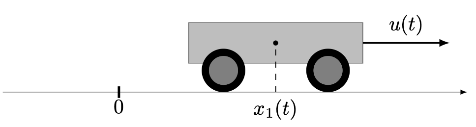
We assume that the mass is constant and unitary and that there is no friction. The dynamics we consider is given by

\[ \dot x_1(t) = x_2(t), \quad \dot x_2(t) = u(t),\quad u(t) \in \R,\]

which is simply the double integrator system. Les us consider a transfer starting at time $t_0 = 0$ and ending at time $t_f = 1$, for which we want to minimise the transfer energy

\[ \frac{1}{2}\int_{0}^{1} u^2(t) \, \mathrm{d}t\]

starting from the condition $x(0) = (-1, 0)$ and with the goal to reach the target $x(1) = (0, 0)$.

First, we need to import the OptimalControl.jl package to define the optimal control problem and NLPModelsIpopt.jl to solve it. We also need to import the Plots.jl package to plot the solution.

using OptimalControl
using NLPModelsIpopt
using Plots

Optimal control problem

Let us define the problem

ocp = @def begin
    t ∈ [0, 1], time
    x ∈ R², state
    u ∈ R, control
    x(0) == [ -1, 0 ]
    x(1) == [ 0, 0 ]
    ẋ(t) == [ x₂(t), u(t) ]
    ∫( 0.5u(t)^2 ) → min
end

Solve and plot

We can solve it simply with:

sol = solve(ocp)

This is Ipopt version 3.14.17, running with linear solver MUMPS 5.7.3.

Number of nonzeros in equality constraint Jacobian...:     3005
Number of nonzeros in inequality constraint Jacobian.:        0
Number of nonzeros in Lagrangian Hessian.............:      251

Total number of variables............................:     1004
                     variables with only lower bounds:        0
                variables with lower and upper bounds:        0
                     variables with only upper bounds:        0
Total number of equality constraints.................:      755
Total number of inequality constraints...............:        0
        inequality constraints with only lower bounds:        0
   inequality constraints with lower and upper bounds:        0
        inequality constraints with only upper bounds:        0

iter    objective    inf_pr   inf_du lg(mu)  ||d||  lg(rg) alpha_du alpha_pr  ls
   0  1.0000000e-01 1.10e+00 2.73e-14   0.0 0.00e+00    -  0.00e+00 0.00e+00   0
   1 -5.0000000e-03 7.36e-02 2.66e-15 -11.0 6.08e+00    -  1.00e+00 1.00e+00h  1
   2  6.0003829e+00 1.78e-15 1.78e-15 -11.0 6.01e+00    -  1.00e+00 1.00e+00h  1

Number of Iterations....: 2

                                   (scaled)                 (unscaled)
Objective...............:   6.0003828724303263e+00    6.0003828724303263e+00
Dual infeasibility......:   1.7763568394002505e-15    1.7763568394002505e-15
Constraint violation....:   1.7763568394002505e-15    1.7763568394002505e-15
Variable bound violation:   0.0000000000000000e+00    0.0000000000000000e+00
Complementarity.........:   0.0000000000000000e+00    0.0000000000000000e+00
Overall NLP error.......:   1.7763568394002505e-15    1.7763568394002505e-15


Number of objective function evaluations             = 3
Number of objective gradient evaluations             = 3
Number of equality constraint evaluations            = 3
Number of inequality constraint evaluations          = 0
Number of equality constraint Jacobian evaluations   = 3
Number of inequality constraint Jacobian evaluations = 0
Number of Lagrangian Hessian evaluations             = 2
Total seconds in IPOPT                               = 1.884

EXIT: Optimal Solution Found.

And plot the solution with:

plot(sol)

State constraint

We add the path constraint

\[x_2(t) \le 1.2.\]

Let us model, solve and plot the optimal control problem with this constraint.

ocp = @def begin

    t ∈ [0, 1], time
    x ∈ R², state
    u ∈ R, control

    x₂(t) ≤ 1.2

    x(0) == [ -1, 0 ]
    x(1) == [ 0, 0 ]

    ẋ(t) == [ x₂(t), u(t) ]

    ∫( 0.5u(t)^2 ) → min

end

sol = solve(ocp)

plot(sol)

Exporting and importing the solution

We can export (or save) the solution in a Julia .jld2 data file and reload it later, and also export a discretised version of the solution in a more portable JSON format. Note that the optimal control problem is needed when loading a solution.

JLD2

using JLD2

export_ocp_solution(sol; filename_prefix="my_solution")

sol_jld = import_ocp_solution(ocp; filename_prefix="my_solution")

println("Objective from computed solution: ", objective(sol))
println("Objective from imported solution: ", objective(sol_jld))

Objective from computed solution: 7.681955388234572
Objective from imported solution: 7.681955388234572

JSON

# load additional modules
using JSON3

export_ocp_solution(sol; filename_prefix="my_solution", format=:JSON)

sol_json = import_ocp_solution(ocp; filename_prefix="my_solution", format=:JSON)

println("Objective from computed solution: ", objective(sol))
println("Objective from imported solution: ", objective(sol_json))

Objective from computed solution: 7.681955388234572
Objective from imported solution: 7.681955388234572