The functional syntax to define an optimal control problem

There are two syntaxes to define an optimal control problem with OptimalControl.jl:

• the standard way is to use the abstract syntax. See for instance basic example for a start or for a comprehensive introduction to the abstract syntax, check this tutorial.
• the old-fashioned functional syntax. In this tutorial with give two examples defined with the functional syntax. For more details please check the Model documentation.

Double integrator: energy minimisation

Let us consider a wagon moving along a rail, whom acceleration can be controlled by a force $u$. We denote by $x = (x_1, x_2)$ the state of the wagon, that is its position $x_1$ and its velocity $x_2$.

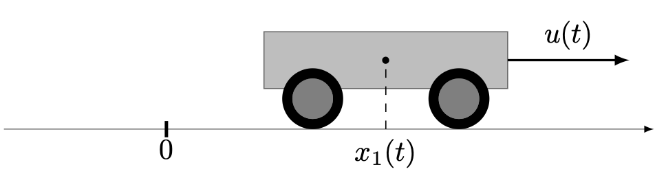
We assume that the mass is constant and unitary and that there is no friction. The dynamics we consider is given by

\[ \dot x_1(t) = x_2(t), \quad \dot x_2(t) = u(t), \quad u(t) \in \R,\]

which is simply the double integrator system. Les us consider a transfer starting at time $t_0 = 0$ and ending at time $t_f = 1$, for which we want to minimise the transfer energy

\[ \frac{1}{2}\int_{0}^{1} u^2(t) \, \mathrm{d}t\]

starting from the condition $x(0) = (-1, 0)$ and with the goal to reach the target $x(1) = (0, 0)$.

Let us define the problem with the functional syntax.

using OptimalControl

ocp = Model()                                   # empty optimal control problem

time!(ocp, t0=0, tf=1)                          # initial and final times
state!(ocp, 2)                                  # dimension of the state
control!(ocp, 1)                                # dimension of the control

constraint!(ocp, :initial; val=[ -1, 0 ])       # initial condition
constraint!(ocp, :final;   val=[  0, 0 ])       # final condition

dynamics!(ocp, (x, u) -> [ x[2], u ])           # dynamics of the double integrator

objective!(ocp, :lagrange, (x, u) -> 0.5u^2)    # cost in Lagrange form

Double integrator: time minimisation

We consider the same optimal control problem where we replace the cost. Instead of minimisation the L2-norm of the control, we consider the time minimisation problem, that is we minimise the final time $t_f$.

ocp = Model(variable=true)                       # variable is true since tf is free

variable!(ocp, 1, :tf)                           # dimension and name of the variable
time!(ocp, t0=0, indf=1)                         # initial time fixed to 0
                                                 # final time free and corresponds to the
                                                 # first component of the variable
state!(ocp, 2, :x, [:q, :v])                     # dimension of the state with names
control!(ocp, 1)                                 # dimension of the control

constraint!(ocp, :variable; lb=0)                # tf ≥ 0
constraint!(ocp, :control; lb=-1, ub=1)          # -1 ≤ u(t) ≤ 1
constraint!(ocp, :initial; val=[ 1, 2 ])         # initial condition
constraint!(ocp, :final;   val=[ 0, 0 ])         # final condition
constraint!(ocp, :state; lb=[-5, -3], ub=[5, 3]) # -5 ≤ q(t) ≤ 5, -3 ≤ v(t) ≤ 3

dynamics!(ocp, (x, u, tf) -> [ x[2], u ])        # dynamics of the double integrator

objective!(ocp, :mayer, (x0, xf, tf) -> tf)      # cost in Mayer form