Zermelo problem, example 2
This example extends the previous Zermelo navigation problem to the case of multiple loss control regions. The state space is now partitioned into two loss control regions and three control regions. This illustrates how the trajectory can visit different loss control regions with potentially different constant control values at each visit.
Problem statement
\[ \left\{ \begin{array}{l} \displaystyle \min - x_1(8), \\[0.5em] \dot{x}_1(t) = x_2(t) + \cos(u(t)), \; \text{for a.e. } t\in [0,8],\\[0.5em] \dot{x}_2(t) = \sin(u(t)), \; \text{for a.e. } t\in [0,8], \\[0.5em] u(t) \in [-\frac{\pi}{2}, \frac{\pi}{2}], \; \text{for a.e. } t\in [0,8], \\[0.5em] x(0) = 0_{\mathbb{R}^2}, \quad x_2(8) = 4,\\[0.5em] \{x \in \mathbb{R}^2 \mid 5 < x_1 < 10 \} \text{ and } \{x \in \mathbb{R}^2 \mid 20 < x_1 < 25 \} \text{ are loss control regions.} \end{array} \right.\]
The partition of $\mathbb{R}^2$ consists of:
- Control regions: $X_1 = \{x \in \mathbb{R}^2 \mid x_1 < 5\}$, $X_3 = \{x \in \mathbb{R}^2 \mid 10 < x_1 < 20\}$, and $X_5 = \{x \in \mathbb{R}^2 \mid x_1 > 25\}$
- Loss control regions: $X_2 = \{x \in \mathbb{R}^2 \mid 5 < x_1 < 10\}$ and $X_4 = \{x \in \mathbb{R}^2 \mid 20 < x_1 < 25\}$
Reformulation for the direct method
\[ \left\{ \begin{array}{l} \displaystyle \min - x_1(8) + \varepsilon \int_0^8 v^2(t)\, \mathrm{d}t + \int_0^8 f_{NC}(x(t))u^2(t)\, \mathrm{d}t, \\[0.5em] \dot{x}_1(t) = f_{C}(x(t)) (x_2(t) + \cos(u(t)))+f_{NC}(x(t)) (x_2(t) + \cos(\lambda(t))), \; \text{for a.e. } t\in [0,8],\\[0.5em] \dot{x}_2(t) = f_{C}(x(t)) \sin(u(t))+f_{NC}(x(t)) \sin(\lambda(t)), \; \text{for a.e. } t\in [0,8], \\[0.5em] \dot{\lambda}(t) = f_{C}(x(t))v(t), \; \text{for a.e. } t\in [0,8], \\[0.5em] u(t)\in [-\frac{\pi}{2}, \frac{\pi}{2}] , \; \text{for a.e. } t\in [0,8], \\[0.5em] x(0) = 0_{\mathbb{R}^2}, \quad x_2(8) = 4,\\[0.5em] \{x \in \mathbb{R}^2 \mid 5 < x_1 < 10 \} \text{ and } \{x \in \mathbb{R}^2 \mid 20 < x_1 < 25 \} \text{ are loss control regions.} \end{array} \right.\]
using Plots
using Plots.PlotMeasures
using OptimalControl
using NLPModelsIpopt
include("smooth.jl")
fNC(x) = fNC_bounded(x, [(5, 10), (20, 25)], 0.05)
plot(fNC, 0, 30, label="fNC")
ε  = 1e-3
tf = 8

@def ocp begin

    t ∈ [ 0, tf ],           time
    q = [ x1, x2, λ ] ∈ R^3, state
    ω = [u, v] ∈ R^2,        control

    x1(0) == 0
    x2(0) == 0
    x2(tf) == 4

    -π/2 ≤ u(t) ≤ π/2
    -π/2 ≤ λ(t) ≤ π/2

    q̇(t) == [
        fNC(x1(t))*(x2(t) + cos(λ(t))) + (1-fNC(x1(t)))*(x2(t) + cos(u(t))),
        fNC(x1(t))*sin(λ(t)) + (1-fNC(x1(t)))*sin(u(t)),
        (1-fNC(x1(t)))*v(t),
    ]

    -x1(tf) + ∫(ε*(v(t))^2+fNC(x1(t))*(u(t))^2)  → min

end
N = 400
sol = solve(ocp; grid_size=N, print_level=4)▫ This is OptimalControl 2.0.0, solving with: collocation → adnlp → ipopt (cpu)
📦 Configuration:
├─ Discretizer: collocation (grid_size = 400)
├─ Modeler: adnlp
└─ Solver: ipopt (print_level = 4)
▫ Total number of variables............................: 2003
variables with only lower bounds: 0
variables with lower and upper bounds: 801
variables with only upper bounds: 0
Total number of equality constraints.................: 1203
Total number of inequality constraints...............: 0
inequality constraints with only lower bounds: 0
inequality constraints with lower and upper bounds: 0
inequality constraints with only upper bounds: 0
Number of Iterations....: 39
(scaled) (unscaled)
Objective...............: -3.0397446657596362e+01 -3.0397446657596362e+01
Dual infeasibility......: 2.2147376987913248e-10 2.2147376987913248e-10
Constraint violation....: 1.2998491172311333e-12 1.2998491172311333e-12
Variable bound violation: 0.0000000000000000e+00 0.0000000000000000e+00
Complementarity.........: 8.1133556427535556e-11 8.1133556427535556e-11
Overall NLP error.......: 2.2147376987913248e-10 2.2147376987913248e-10
Number of objective function evaluations = 42
Number of objective gradient evaluations = 40
Number of equality constraint evaluations = 42
Number of inequality constraint evaluations = 0
Number of equality constraint Jacobian evaluations = 40
Number of inequality constraint Jacobian evaluations = 0
Number of Lagrangian Hessian evaluations = 39
Total seconds in IPOPT = 6.711
EXIT: Optimal Solution Found.plot(sol; layout=:group, size=(800, 300))
tt2 = (0:N+1) * (tf/(N+1))
y1(t) = state(sol)(t)[1]
y2(t) = state(sol)(t)[2]
μ(t)  = state(sol)(t)[3]
v(t)  = control(sol)(t)[1]
q1(t) = costate(sol)(t)[1]
q2(t) = costate(sol)(t)[2]
plot(y1, y2, 0, tf, label="optimal trajectory", color="blue", linewidth=2)
plot!([5, 5], [0, 6], color=:black, label = false, linewidth=2)
plot!([10, 10], [0,6], color=:black, label = false, linewidth=2)
plot!([20, 20], [0, 6], color=:black, label = false, linewidth=2)
plot!([25, 25], [0,6], color=:black, label = false, linewidth=2)
plot( tt2, v, label="optimal control", color="red", linewidth=2)
plot!(tt2, μ, label="state λ", color="green", linewidth=2)
plot( tt2, q1, label="costate p1", color="purple", linewidth=2)
plot!(tt2, q2, label="costate p2", color="violet", linewidth=2)
# Find the crossing times based on conditions for x1
s1_index = findfirst(t -> y1(t) > 5, tt2)
s2_index = nothing
s3_index = nothing
s4_index = nothing

# If t1 is found, find the next crossing times
if s1_index !== nothing
    s2_index = findfirst(t -> y1(t) > 10, tt2[s1_index+1:end])
    s2_index = s2_index !== nothing ? s2_index + s1_index : nothing
end

if s2_index !== nothing
    s3_index = findfirst(t -> y1(t) > 20, tt2[s2_index+1:end])
    s3_index = s3_index !== nothing ? s3_index + s2_index : nothing
end

if s3_index !== nothing
    s4_index = findfirst(t -> y1(t) > 25, tt2[s3_index+1:end])
    s4_index = s4_index !== nothing ? s4_index + s3_index : nothing
end

# Convert indices to times
s1 = s1_index !== nothing ? tt2[s1_index] : "No such t1 found"
s2 = s2_index !== nothing ? tt2[s2_index] : "No such t2 found"
s3 = s3_index !== nothing ? tt2[s3_index] : "No such t3 found"
s4 = s4_index !== nothing ? tt2[s4_index] : "No such t4 found"

println("First crossing time: ",  s1)
println("Second crossing time: ", s2)
println("Third crossing time: ",  s3)
println("Fourth crossing time: ", s4)
First crossing time: 2.9925187032418954
Second crossing time: 4.26932668329177
Third crossing time: 6.104738154613466
Fourth crossing time: 6.942643391521197# extract constant values of λ
b1 = μ((s1+s2)/2)
b2 = μ((s3+s4)/2)
println("First constant value of λ: ", b1)
println("Second constant value of λ: ", b2)First constant value of λ: 1.1742385770439288
Second constant value of λ: -0.3857077728403158jmp1 = q1(s1+0.1) - q1(s1-0.1)
jmp2 = q1(s2+0.1) - q1(s2-0.1)
jmp3 = q1(s3+0.1) - q1(s3-0.1)
jmp4 = q1(s4+0.1) - q1(s4-0.1)
println("p1(t1+) - p1(t1-) = ", jmp1)
println("p1(t2+) - p1(t2-) = ", jmp2)
println("p1(t3+) - p1(t3-) = ", jmp3)
println("p1(t4+) - p1(t4-) = ", jmp4)p1(t1+) - p1(t1-) = 0.018787725087285434
p1(t2+) - p1(t2-) = -0.04736806156070772
p1(t3+) - p1(t3-) = 0.012958574913464416
p1(t4+) - p1(t4-) = -0.026648746402953893Analysis of the direct method results
The direct method shows that the optimal trajectory visits both loss control regions $X_2$ and $X_4$ with two different constant control values in $(-\frac{\pi}{2}, \frac{\pi}{2})$. The adjoint vector $p_1$ exhibits discontinuity jumps at each of the four crossing times.
Indirect Method
Based on the direct method results, we deduce that the optimal solution $(x^*, u^*)$ has five arcs:
- Feedback arc (in $X_1$)
- Constant arc (in $X_2$): first constant value
- Feedback arc (in $X_3$)
- Constant arc (in $X_4$): second constant value (potentially different from the first)
- Feedback arc (in $X_5$)
Since the regions are vertical, $p_2$ is continuous over $[0,8]$, whereas $p_1$ may have jumps at crossing times. From the Hamiltonian maximization condition in control regions, we have $u^*(t) = \arctan(p_2(t))$.
using NonlinearSolve
using OrdinaryDiffEq
using Animations
# Dynamics
function F(x, u)
return [x[2] + cos(u), sin(u)]
end
function G(λ)
return [sin(λ), -cos(λ)]
end
# Hamiltonian: permanent region
H1(x, u, p) = p' * F(x, u) # pseudo-Hamiltonian
u11(x, p) = atan(p[2]/p[1]) # maximizing control
Hc(x, p) = H1(x, u11(x, p), p) # Hamiltonian
# Flow
fc = Flow(OptimalControl.Hamiltonian(Hc))
# Hamiltonian: control loss region
H2(x, λ, y, p) = p' * F(x, λ) + y* p' *G(λ) # pseudo-Hamiltonian
Hcl(X, P) = H2(X[1:2], X[3], X[4], P[1:2]) # Hamiltonian
# Flow
fcl = Flow(OptimalControl.Hamiltonian(Hcl))# parameters
t0 = 0
tf = 8
x2f = 4
x0 = [0, 0]# Shooting function
function shoot2(p0, tt1, tt2, tt3, tt4, λ1, λ3, j1, j2, j3, j4)
pλ0 = 0
qy0 = 0
y1, q1 = fc(t0, x0, p0, tt1)
Y2, Q2 = fcl(tt1, [y1; λ1; 0], [q1 - [j1 , 0]; pλ0 ; qy0], tt2)
y3, q3 = fc(tt2, Y2[1:2], Q2[1:2] - [j2 , 0], tt3)
Y4, Q4 = fcl(tt3, [y3; λ3; 0], [q3 - [j3 , 0]; pλ0 ; qy0], tt4)
yf, qf = fc(tt4, Y4[1:2], Q4[1:2] - [j4 , 0], tf)
s = zeros(eltype(p0), 12)
s[1] = yf[2] - x2f # target
s[2] = qf[1] - 1 # transversality condition
s[3] = y1[1] - 2 # first crossing
s[4] = Y2[1] - 16 # second crossing
s[5] = y3[1] - 20 # first crossing
s[6] = Y4[1] - 25 # second crossing
s[7] = Q2[4] # averaged gradient condition1
s[8] = Q4[4] # averaged gradient condition2
v_temp = u11(y1, q1)
s[9] = j1 - (q1[1]*(cos(λ1) - cos(v_temp)) +
q1[2]*(sin(λ1) - sin(v_temp)))/(y1[2] + cos(λ1)) # jump 1
v_temp = u11(Y2[1:2], Q2[1:2])
s[10] = j2 - (Q2[1]*(cos(v_temp) - cos(λ1)) +
Q2[2]*(sin(v_temp) - sin(λ1)))/(Y2[2]+cos(v_temp)) # jump 2
v_temp = u11(y3, q3)
s[11] = j3 - (q3[1]*(cos(λ3) - cos(v_temp)) +
q3[2]*(sin(λ3) - sin(v_temp)))/(y3[2] + cos(λ3)) # jump 3
v_temp = u11(Y4[1:2], Q4[1:2])
s[12] = j4 - (Q4[1]*(cos(v_temp) - cos(λ3)) +
Q4[2]*(sin(v_temp) - sin(λ3)))/(Y4[2]+cos(v_temp)) # jump 4
return s
end# auxiliary function with aggregated inputs
nle! = (ξ, λ) -> shoot2(ξ[1:2], ξ[3], ξ[4], ξ[5], ξ[6], ξ[7], ξ[8], ξ[9], ξ[10], ξ[11], ξ[12])
# initial guess
ξ_guess =[q1(0), q2(0), s1, s2, s3, s4, b1, b2, jmp1, jmp2, jmp3, jmp4]
prob = NonlinearProblem(nle!, ξ_guess)indirect_sol = solve(prob, SimpleNewtonRaphson(); abstol=1e-8, reltol=1e-8, show_trace=Val(true))# retrieves solution
qq0 = indirect_sol[1:2]
ss1 = indirect_sol[3]
ss2 = indirect_sol[4]
ss3 = indirect_sol[5]
ss4 = indirect_sol[6]
bb1 = indirect_sol[7]
bb2 = indirect_sol[8]
j11 = indirect_sol[9]
j22 = indirect_sol[10]
j33 = indirect_sol[11]
j44 = indirect_sol[12]# jumps from indirect solution
println("jumps from indirect solution")
println("p1(t1+) - p1(t1-) = ", j11)
println("p1(t2+) - p1(t2-) = ", j22)
println("p1(t3+) - p1(t3-) = ", j33)
println("p1(t4+) - p1(t4-) = ", j44)jumps from indirect solution
p1(t1+) - p1(t1-) = -0.031233366896828384
p1(t2+) - p1(t2-) = 0.044786964257001016
p1(t3+) - p1(t3-) = -0.011471041147338533
p1(t4+) - p1(t4-) = 0.009189735902405774qa0 = 0
qb0 = 0
qy0 = 0
qz0 = 0
ode_sol = fc((t0, ss1), x0, qq0, saveat=0.1)
ttt1 = ode_sol.t ;
yy1 = [ ode_sol[1:2, j] for j in 1:size(ttt1, 1) ]
qq1 = [ ode_sol[3:4, j] for j in 1:size(ttt1, 1) ]
vv1 = u11.(yy1, qq1)
ode_sol = fcl((ss1, ss2), [yy1[end] ; bb1 ; 0.0], [qq1[end] - [ j11, 0.]; qa0 ; qy0], saveat=0.1)
ttt2 = ode_sol.t
yy2 = [ ode_sol[1:2, j] for j in 1:size(ttt2, 1) ]
qq2 = [ ode_sol[5:6, j] for j in 1:size(ttt2, 1) ]
vv2 = bb1.*ones(length(ttt2))
ode_sol = fc((ss2, ss3), yy2[end], qq2[end] - [j22, 0.], saveat=0.1)
ttt3 = ode_sol.t
yy3 = [ ode_sol[1:2, j] for j in 1:size(ttt3, 1) ]
qq3 = [ ode_sol[3:4, j] for j in 1:size(ttt3, 1) ]
vv3 = u11.(yy3, qq3)
ode_sol = fcl((ss3, ss4), [yy3[end] ; b2 ; 0.0], [qq3[end] - [j33, 0.]; qb0 ; qz0], saveat=0.1)
ttt4 = ode_sol.t
yy4 = [ ode_sol[1:2, j] for j in 1:size(ttt4, 1) ]
qq4 = [ ode_sol[5:6, j] for j in 1:size(ttt4, 1) ]
vv4 = bb2.*ones(length(ttt4))
ode_sol = fc((ss4, tf), yy4[end], qq4[end]- [j44, 0.], saveat=0.1)
ttt5 = ode_sol.t
yy5 = [ ode_sol[1:2, j] for j in 1:size(ttt5, 1) ]
qq5 = [ ode_sol[3:4, j] for j in 1:size(ttt5, 1) ]
vv5 = u11.(yy5, qq5)
ttt = [ ttt1 ; ttt2 ; ttt3 ; ttt4 ; ttt5]
yyy = [ yy1 ; yy2 ; yy3 ; yy4 ; yy5 ]
qqq = [ qq1 ; qq2 ; qq3 ; qq4 ; qq5 ]
vvv = [ vv1 ; vv2 ; vv3 ; vv4 ; vv5 ]
m = length(ttt)
yy1 = [ yyy[i][1] for i=1:m ]
yy2 = [ yyy[i][2] for i=1:m ]
qq1 = [ qqq[i][1] for i=1:m ]
qq2 = [ qqq[i][2] for i=1:m ]plot(yy1, yy2, label="optimal trajectory", legend=false, linecolor=:blue, linewidth=2)
plot!([5, 5], [0, 6], color=:black, label = false, linewidth=2)
plot!([10, 10], [0,6], color=:black, label = false, linewidth=2)
plot!([20, 20], [0, 6], color=:black, label = false, linewidth=2)
plot!([25, 25], [0,6], color=:black, label = false, linewidth=2)
plot(ttt, vvv, label="optimal control" ,linecolor=:red ,linewidth=2)
plot(ttt,  qq1, label="costate p1", linecolor=:purple, linewidth=2)
plot!(ttt, qq2, label="costate p2", linecolor=:violet, linewidth=2)
# create an animation
animy = @animate for i = 1:length(ttt)
    plot(yy1[1:i], yy2[1:i],  xlim=(0.,31.), ylim=(-0.,5.5), label="optimal trajectory",
        linecolor=:blue,  linewidth=2, legend=:topleft)
    scatter!([yy1[i]], [yy2[i]], markersize=4, marker=:circle, color=:black, label=false)
    plot!([5,   5], [0, 6], color=:black, label = false, linewidth=2)
    plot!([10, 10], [0, 6], color=:black, label = false, linewidth=2)
    plot!([20, 20], [0, 6], color=:black, label = false, linewidth=2)
    plot!([25, 25], [0, 6], color=:black, label = false, linewidth=2)
end

animv = @animate for i = 1:length(ttt)
    plot(ttt[1:i], vvv[1:i], xlim=(0.,8.), ylim=(-pi/2,pi/2), label="optimal control",
        linecolor=:red, linewidth=2)
end

animq1 = @animate for i = 1:length(ttt)
    plot(ttt[1:i], qq1[1:i], xlim=(0.,8.), ylim=(0.,2.) , label="costate p1",
        linecolor=:purple, linewidth=2)
end

animq2 = @animate for i = 1:length(ttt)
    plot(ttt[1:i], qq2[1:i], xlim=(0.,8.), ylim=(-2.2,6.), label="costate p2",
        linecolor=:violet, linewidth=2)
end
gif(animy, "zer2_y.gif", fps = 10)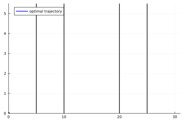
gif(animv, "zer2_v.gif", fps = 10)
gif(animq1, "zer2_q1.gif", fps = 10)