Zermelo navigation problem, example 1
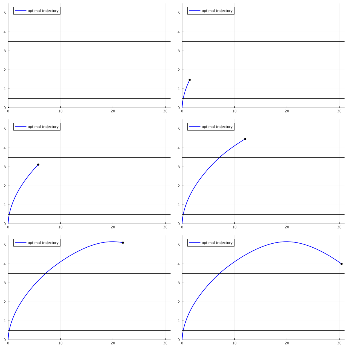
This example illustrates a Zermelo-type navigation problem with a single loss control region. The state space is partitioned into one loss control region (where $0.5 < x_2 < 3.5$) and two control regions. When the trajectory enters the loss control region, the control must remain constant, though its value is optimized and can differ at each visit.
Problem statement
\[ \left\{ \begin{array}{l} \displaystyle \min - x_1(8), \\[0.5em] \dot{x}_1(t) = x_2(t) + \cos(u(t)), \; \text{for a.e. } t\in [0,8],\\[0.5em] \dot{x}_2(t) = \sin(u(t)), \; \text{for a.e. } t\in [0,8], \\[0.5em] u(t) \in [-\frac{\pi}{2}, \frac{\pi}{2}], \; \text{for a.e. } t\in [0,8], \\[0.5em] x(0) = 0_{\mathbb{R}^2}, \quad x_2(8) = 4,\\[0.5em] \{x \in \mathbb{R}^2 \mid 0.5 < x_2 < 3.5 \} \text{ is a loss control region.} \end{array} \right.\]
The partition of $\mathbb{R}^2$ consists of:
- Control regions: $X_1 = \{x \in \mathbb{R}^2 \mid x_2 < 0.5\}$ and $X_3 = \{x \in \mathbb{R}^2 \mid x_2 > 3.5\}$ (where control can change at any time)
- Loss control region: $X_2 = \{x \in \mathbb{R}^2 \mid 0.5 < x_2 < 3.5\}$ (where control must remain constant)
Reformulation for the direct method
\[ \left\{ \begin{array}{l} \displaystyle \min - x_1(8) + \varepsilon\int_0^8 v^2(t)\, \mathrm{d}t + \int_0^8 f_{NC}(x(t))u^2(t)\, \mathrm{d}t, \\[0.5em] \dot{x}_1(t) = f_{C}(x(t))(x_2(t) + \cos(u(t))) + f_{NC}(x_2(t) + \cos(\lambda(t))), \; \text{for a.e. } t\in [0,8],\\[0.5em] \dot{x}_2(t) = f_{C}(x(t))\sin(u(t)) + f_{NC}(x(t))\sin(\lambda(t)), \; \text{for a.e. } t\in [0,8], \\[0.5em] \dot{\lambda}(t) = f_{C}(x(t))v^2(t), \; \text{for a.e. } t\in [0,8], \\[0.5em] u(t) \in [-\frac{\pi}{2}, \frac{\pi}{2}], \; \text{for a.e. } t\in [0,8], \\[0.5em] x(0) = 0_{\mathbb{R}^2}, \quad x_2(8) = 4,\\[0.5em] \{x \in \mathbb{R}^2 \mid 0.5 < x_2 < 3.5 \} \text{ is a loss control region.} \end{array} \right.\]
using Plots
using Plots.PlotMeasures
using OptimalControl
using NLPModelsIpopt
include("smooth.jl")
fNC(x) = fNC_bounded(x, [(0.5, 3.5)], 0.01)
plot(fNC, 0, 5, label="fNC")ε = 1e-3
tf = 8
ocp = @def begin
t ∈ [ 0, tf ], time
q = ( x1, x2, λ ) ∈ R^3, state
ω = (u, v) ∈ R^2, control
x1(0) == 0
x2(0) == 0
x2(tf) == 4
-π/2 ≤ u(t) ≤ π/2
-π/2 ≤ λ(t) ≤ π/2
q̇(t) == [
fNC(x2(t))*(x2(t) + cos(λ(t))) + (1-fNC(x2(t)))*(x2(t) + cos(u(t))),
fNC(x2(t))*sin(λ(t)) +(1-fNC(x2(t)))*sin(u(t)),
(1-fNC(x2(t)))*v(t),
]
-x1(tf) + ∫(ε*(v(t))^2+fNC(x2(t))*(u(t))^2) → min
endN = 500
sol = solve(ocp; grid_size=N, print_level=4)▫ This is OptimalControl 2.0.0, solving with: collocation → adnlp → ipopt (cpu)
📦 Configuration:
├─ Discretizer: collocation (grid_size = 500)
├─ Modeler: adnlp
└─ Solver: ipopt (print_level = 4)
▫ Total number of variables............................: 2503
variables with only lower bounds: 0
variables with lower and upper bounds: 1001
variables with only upper bounds: 0
Total number of equality constraints.................: 1503
Total number of inequality constraints...............: 0
inequality constraints with only lower bounds: 0
inequality constraints with lower and upper bounds: 0
inequality constraints with only upper bounds: 0
Number of Iterations....: 62
(scaled) (unscaled)
Objective...............: -3.0402363910579702e+01 -3.0402363910579702e+01
Dual infeasibility......: 1.6057483120945903e-10 1.6057483120945903e-10
Constraint violation....: 5.6719073882049997e-12 5.6719073882049997e-12
Variable bound violation: 0.0000000000000000e+00 0.0000000000000000e+00
Complementarity.........: 2.1102167127080718e-11 2.1102167127080718e-11
Overall NLP error.......: 1.6057483120945903e-10 1.6057483120945903e-10
Number of objective function evaluations = 63
Number of objective gradient evaluations = 63
Number of equality constraint evaluations = 63
Number of inequality constraint evaluations = 0
Number of equality constraint Jacobian evaluations = 63
Number of inequality constraint Jacobian evaluations = 0
Number of Lagrangian Hessian evaluations = 62
Total seconds in IPOPT = 7.074
EXIT: Optimal Solution Found.plot(sol; layout=:group, size=(800, 300))tt1 = (0:N+1) * (tf/(N+1))
x1(t) = state(sol)(t)[1]
x2(t) = state(sol)(t)[2]
λ(t) = state(sol)(t)[3]
u(t) = control(sol)(t)[1]
p1(t) = costate(sol)(t)[1]
p2(t) = costate(sol)(t)[2]
a = λ(tf)plot(x1, x2, 0, tf, label="optimal trajectory", color="blue", linewidth=2)
plot!([0, 31], [0.5, 0.5], color=:black, label = false, linewidth=2)
plot!([0, 31], [3.5, 3.5], color=:black, label = false, linewidth=2)plot( u, 0, tf, label="optimal control", color="red", linewidth=2)
plot!(λ, 0, tf, label="state λ", color="green", linewidth=2)plot( p1, 0, tf, label="costate p1", color="purple", linewidth=2)
plot!(p2, 0, tf, label="costate p2", color="violet", linewidth=2)# Find the first crossing time
t1_index = findfirst(t -> x2(t) ≥ 0.5, tt1)
# If t1 is found, find the next crossing time
if t1_index !== nothing
t1 = tt1[t1_index]
t2_index = findfirst(t -> x2(t) ≥ 3.5, tt1[t1_index+1:end])
t2_index = t2_index !== nothing ? t2_index + t1_index : nothing
t2 = t2_index !== nothing ? tt1[t2_index] : "No such t2 found"
else
t1 = "No such t1 found"
t2 = "No such t2 found"
end
println("first crossing time: ", t1)
println("second crossing time: ", t2)first crossing time: 0.5109780439121756
second crossing time: 3.6087824351297404jmp1 = p2(t1+0.1) - p2(t1-0.1)
jmp2 = p2(t2+0.1) - p2(t2-0.1)
println("p2(t1+) - p2(t1-) = ", jmp1)
println("p2(t2+) - p2(t2-) = ", jmp2)p2(t1+) - p2(t1-) = -0.11079799024762593
p2(t2+) - p2(t2-) = -0.22685627203858472Analysis of the direct method results
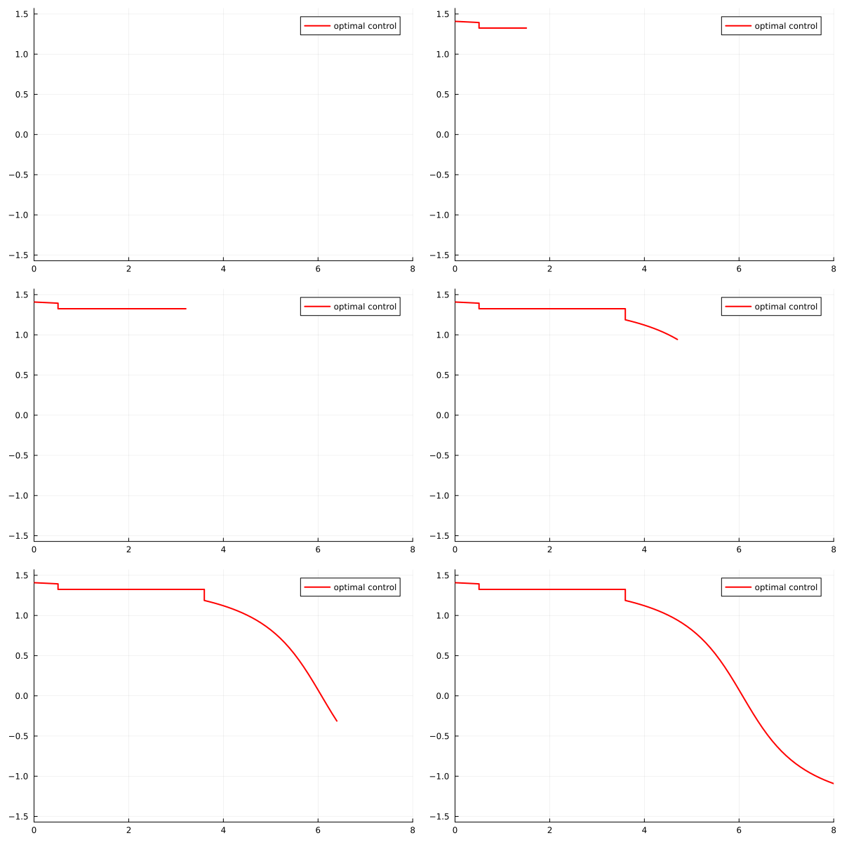
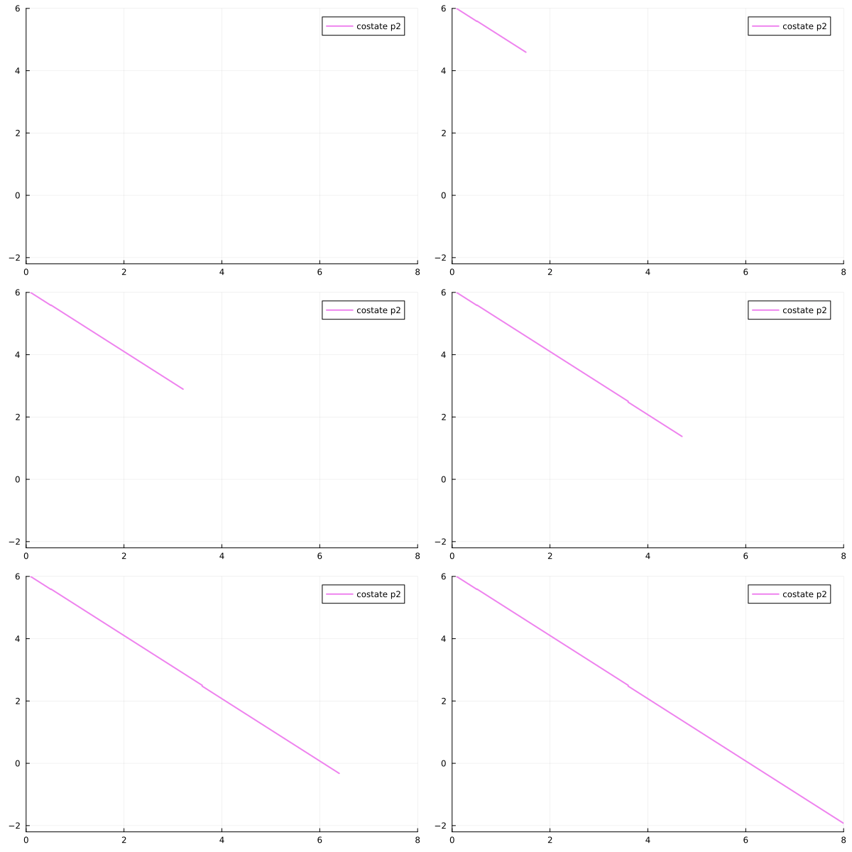
The direct method reveals that the optimal trajectory visits the loss control region $X_2$ once with a constant control value $\lambda \in (-\frac{\pi}{2}, \frac{\pi}{2})$. The adjoint vector $p_2$ exhibits discontinuity jumps at each crossing time, which is characteristic of spatially heterogeneous optimal control problems.
Indirect Method
Based on the direct method results, we deduce that the optimal solution $(x^*, u^*)$ has three arcs:
- Feedback arc (in $X_1$): the control is expressed as $u^*(t) = \arctan(p_2(t))$ using the Hamiltonian maximization condition
- Constant arc (in $X_2$): the control takes a constant value in $(-\frac{\pi}{2}, \frac{\pi}{2})$
- Feedback arc (in $X_3$): again $u^*(t) = \arctan(p_2(t))$
Note that the adjoint vector $p_1$ is continuous over $[0,8]$ since the interfaces between regions are horizontal lines. Only $p_2$ may have jumps at crossing times.
using NonlinearSolve
using OrdinaryDiffEq
using Animations
# Dynamics
function F(x, u)
return [x[2] + cos(u), sin(u)]
end
function G(λ)
return [sin(λ), -cos(λ)]
end
# Hamiltonian: permanent region
H1(x, u, p) = p' * F(x, u) # pseudo-Hamiltonian
u11(x, p) = atan(p[2]/p[1]) # maximizing control
Hc(x, p) = H1(x, u11(x, p) , p ) # Hamiltonian
# Flow
fc = Flow(OptimalControl.Hamiltonian(Hc))
# Hamiltonian: control loss region
H2(x, λ, y, p) = p' * F(x, λ) + y* p' *G(λ) # pseudo-Hamiltonian
Hcl(X, P) = H2(X[1:2], X[3], X[4], P[1:2]) # Hamiltonian
# Flow
fcl = Flow(OptimalControl.Hamiltonian(Hcl))# parameters
t0 = 0
tf = 8
x2f = 4
x0 = [0, 0]function shoot1(p0, tt1, tt2, λ, jump1, jump2)
pλ0 = 0
py0 = 0
x1, p1 = fc(t0, x0, p0, tt1)
X2, P2 = fcl(tt1, [x1; λ; 0], [p1 - [0, jump1]; pλ0; py0], tt2) # augmented flow
xf, pf = fc(tt2, X2[1:2], P2[1:2] - [0, jump2], tf)
s = zeros(eltype(p0), 7)
s[1] = xf[2] - x2f # target
s[2] = pf[1] - 1.0 # transversality condition
s[3] = x1[2] - 0.5 # first crossing
s[4] = X2[2] - 3.5 # second crossing
s[5] = P2[4] # averaged gradient condition
s[6] = jump1 - (p1[1]*(cos(λ) - cos(u11(x1, p1))) +
p1[2]*(sin(λ) - sin(u11(x1, p1))))/(sin(λ)) #jump 1
s[7] = jump2 - (P2[1]*(cos(u11(X2[1:2], P2[1:2])) - cos(λ)) +
P2[2]*(sin(u11(X2[1:2], P2[1:2])) - sin(λ)))/(sin(u11(X2[1:2], P2[1:2]))) #jump 2
return s
end# auxiliary function with aggregated inputs
nle! = (ξ, λ) -> shoot1(ξ[1:2], ξ[3], ξ[4], ξ[5], ξ[6], ξ[7])
# initial guess
ξ_guess = [p1(0), p2(0), t1, t2, a, jmp1, jmp2]
prob = NonlinearProblem(nle!, ξ_guess)indirect_sol = solve(prob, SimpleNewtonRaphson(); abstol=1e-8, reltol=1e-8, show_trace=Val(true))# retrieves solution
pp0 = indirect_sol[1:2]
tt1 = indirect_sol[3]
tt2 = indirect_sol[4]
aa = indirect_sol[5]
jmp11 = indirect_sol[6]
jmp22 = indirect_sol[7]# jumps from indirect solution
println("jumps from indirect solution")
println("p2(t1+) - p2(t1-) = ", jmp11)
println("p2(t2+) - p2(t2-) = ", jmp22)jumps from indirect solution
p2(t1+) - p2(t1-) = -0.012281989939688712
p2(t2+) - p2(t2-) = 0.027541288724051163ode_sol = fc((t0, tt1), x0, pp0, saveat=0.1)
ttt1 = ode_sol.t
xx1 = [ ode_sol[1:2, j] for j in 1:size(ttt1, 1) ]
pp1 = [ ode_sol[3:4, j] for j in 1:size(ttt1, 1) ]
uu1 = u11.(xx1, pp1)
pλ0 = 0.
py0 = 0.
ode_sol = fcl((tt1, tt2), [xx1[end] ; aa ; 0.0], [pp1[end] - [0. , jmp11]; pλ0 ; py0], saveat=0.1)
ttt2 = ode_sol.t
xx2 = [ ode_sol[1:2, j] for j in 1:size(ttt2, 1) ]
pp2 = [ ode_sol[5:6, j] for j in 1:size(ttt2, 1) ]
uu2 = a.*ones(length(ttt2)) ;
ode_sol = fc((tt2, tf), xx2[end], pp2[end] - [0. , jmp22], saveat=0.1)
ttt3 = ode_sol.t
xx3 = [ ode_sol[1:2, j] for j in 1:size(ttt3, 1) ]
pp3 = [ ode_sol[3:4, j] for j in 1:size(ttt3, 1) ]
uu3 = u11.(xx3, pp3)
tsol = [ ttt1 ; ttt2 ; ttt3 ]
xsol = [ xx1 ; xx2 ; xx3 ]
psol = [ pp1 ; pp2 ; pp3 ]
usol = [ uu1 ; uu2 ; uu3 ]
m = length(tsol)
x11 = [ xsol[i][1] for i=1:m ]
x22 = [ xsol[i][2] for i=1:m ]
p11 = [ psol[i][1] for i=1:m ]
p22 = [ psol[i][2] for i=1:m ]plot(x11, x22, label="optimal trajectory", legend=false, linecolor=:blue, linewidth=2)
hline!([(0., 0.5), (31., 0.5)], linecolor=:black, linewidth=2, label=false)
hline!([(0., 3.5), (31., 3.5)], linecolor=:black, linewidth=2, label=false)plot(tsol, usol, label="optimal control" ,linecolor=:red ,linewidth=2)plot(tsol, p11, label="costate p1", linecolor=:purple, linewidth=2)
plot!(tsol, p22, label="costate p2", linecolor=:violet, linewidth=2)# create an animation
animx = @animate for i = 1:length(tsol)
plot(x11[1:i], x22[1:i], xlim=(0.,31.), ylim=(-0.,5.5), label="optimal trajectory",
linecolor=:blue, linewidth=2, legend=:topleft)
scatter!([x11[i]], [x22[i]], markersize=4, marker=:circle, color=:black, label=false)
plot!([0, 31], [0.5, 0.5], color=:black, label=false, linewidth=2)
plot!([0, 31], [3.5, 3.5], color=:black, label=false, linewidth=2)
end
animu = @animate for i = 1:length(tsol)
plot(tsol[1:i], usol[1:i], xlim=(0.,8.), ylim=(-pi/2,pi/2), label="optimal control",
linecolor=:red, linewidth=2)
end
animp1 = @animate for i = 1:length(tsol)
plot(tsol[1:i], p11[1:i], xlim=(0.,8.), ylim=(0.,2.) , label="costate p1",
linecolor=:purple, linewidth=2)
end
animp2 = @animate for i = 1:length(tsol)
plot(tsol[1:i], p22[1:i], xlim=(0.,8.), ylim=(-2.2,6.), label="costate p2",
linecolor=:violet, linewidth=2)
end# display the animation
gif(animx, "zer1_x.gif", fps = 10)
gif(animu, "zer1_u.gif", fps = 10)
gif(animp2, "zer1_p2.gif", fps = 10)