Numerical developments to solve optimal control problems in Julia
Jean-Baptiste Caillau, Olivier Cots, Joseph Gergaud, Pierre Martinon, Sophia Sed

What it's about
- Nonlinear optimal control of ODEs:
\[g(x(t_0),x(t_f)) + \int_{t_0}^{t_f} f^0(x(t), u(t))\, \mathrm{d}t \to \min\]
subject to
\[\dot{x}(t) = f(x(t), u(t)),\quad t \in [t_0, t_f]\]
plus boundary, control and state constraints
- Our core interests: numerical & geometrical methods in control, applications
- Why Julia: fast (+ JIT), strongly typed, high-level (AD, macros), fast optimisation and ODE solvers available, rapidly growing community
What is important to solve such a problem numerically?
Syntax matters
Do more...
rewrite in OptimalControl.jl DSL the free time problem below as a problem with fixed final time using:
- a change time from t to s = t / tf
- tf as an additional state variable subject to dtf / ds = 0
ocp = @def begin
    tf ∈ R,          variable
    t ∈ [0, tf],     time
    x = (q, v) ∈ R², state
    u ∈ R,           control
    -1 ≤ u(t) ≤ 1
    q(0)  == -1
    v(0)  == 0
    q(tf) == 0
    v(tf) == 0
    ẋ(t) == [v(t), u(t)]
    tf → min
end
ocp_fixed = @def begin
# Fixed time domain
s ∈ [0, 1], time
# Augmented state: (position, velocity, final_time)
y = (q, v, tf) ∈ R³, state
# Control
u ∈ R, control
# Transformed dynamics (multiply by tf due to ds = dt/tf)
∂(q)(s) == tf(s) * v(s)
∂(v)(s) == tf(s) * u(s)
∂(tf)(s) == 0
# Initial conditions
q(0) == -1
v(0) == 0
# tf(0) is free (no initial condition needed)
# Final conditions
q(1) == 0
v(1) == 0
# tf(1) is what we minimize
# Control constraints
-1 ≤ u(s) ≤ 1
# Cost: minimize final time
tf(1) → min
endPerformance matters
- Discretising an OCP into an NLP: $h_i := t_{i+1}-t_i$,
\[g(X_0,X_N) + \sum_{i=0}^{N} h_i f^0(X_i,U_i) \to \min\]
subject to
\[X_{i+1} - X_i - h_i f(X_i, U_i) = 0,\quad i = 0,\dots,N-1\]
plus other constraints on $X := (X_i)_{i=0,N}$ and $U := (U_i)_{i=0,N}$ such as boundary and path (state and / or control) constraints :
\[b(t_0, X_0, t_N, X_N) = 0\]
\[c(X_i, U_i) \leq 0,\quad i = 0,\dots,N\]
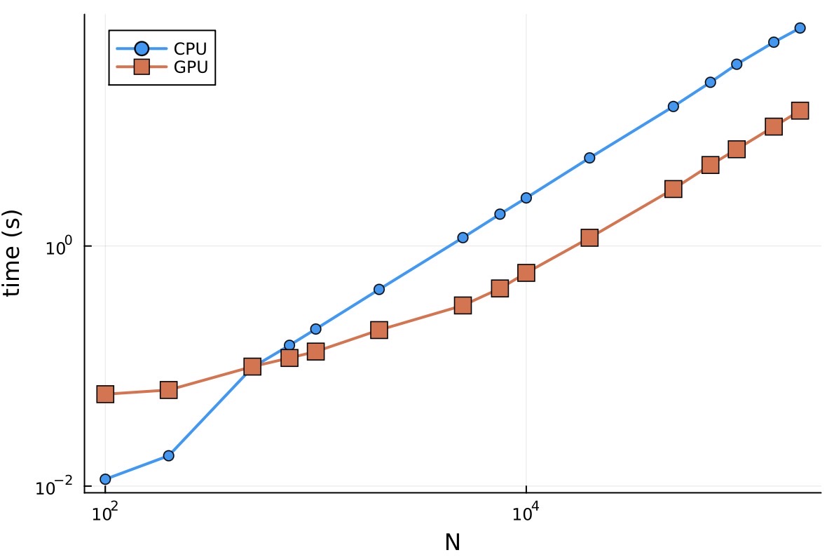
- SIMD parallelism ($f_0$, $f$, $g$) + sparsity: Kernels for GPU (KernelAbstraction.jl) and sparse linear algebra (CUDSS.jl)
- Modelling and optimising for GPU: ExaModels.jl + MadNLP.jl, with built-in AD
- Compile into an ExaModel (one pass compiler, syntax + semantics)
Solving (MadNLP + CUDSS)
This is MadNLP version v0.8.7, running with cuDSS v0.4.0

Number of nonzeros in constraint Jacobian............:    12005
Number of nonzeros in Lagrangian Hessian.............:     9000

Total number of variables............................:     4004
                     variables with only lower bounds:        0
                variables with lower and upper bounds:        0
                     variables with only upper bounds:        0
Total number of equality constraints.................:     3005
Total number of inequality constraints...............:        0
        inequality constraints with only lower bounds:        0
   inequality constraints with lower and upper bounds:        0
        inequality constraints with only upper bounds:        0

iter    objective    inf_pr   inf_du lg(mu)  ||d||  lg(rg) alpha_du alpha_pr  ls
   0  1.0000000e-01 1.10e+00 1.00e+00  -1.0 0.00e+00    -  0.00e+00 0.00e+00   0
   1  1.0001760e-01 1.10e+00 3.84e-03  -1.0 6.88e+02  -4.0 1.00e+00 2.00e-07h  2
   2 -5.2365072e-03 1.89e-02 1.79e-07  -1.0 6.16e+00  -4.5 1.00e+00 1.00e+00h  1
   3  5.9939621e+00 2.28e-03 1.66e-04  -3.8 6.00e+00  -5.0 9.99e-01 1.00e+00h  1
   4  5.9996210e+00 2.94e-06 8.38e-07  -3.8 7.70e-02    -  1.00e+00 1.00e+00h  1

Number of Iterations....: 4

                                   (scaled)                 (unscaled)
Objective...............:   5.9996210189633494e+00    5.9996210189633494e+00
Dual infeasibility......:   8.3756005011360529e-07    8.3756005011360529e-07
Constraint violation....:   2.9426923277963834e-06    2.9426923277963834e-06
Complementarity.........:   2.0007459547789288e-06    2.0007459547789288e-06
Overall NLP error.......:   2.9426923277963834e-06    2.9426923277963834e-06

Number of objective function evaluations             = 6
Number of objective gradient evaluations             = 5
Number of constraint evaluations                     = 6
Number of constraint Jacobian evaluations            = 5
Number of Lagrangian Hessian evaluations             = 4
Total wall-clock secs in solver (w/o fun. eval./lin. alg.)  =  0.072
Total wall-clock secs in linear solver                      =  0.008
Total wall-clock secs in NLP function evaluations           =  0.003
Total wall-clock secs                                       =  0.083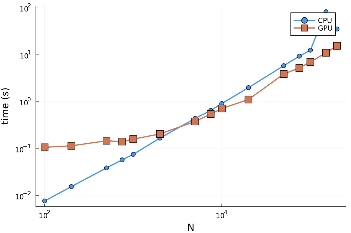
- Quadrotor, H100 run
Maths matters
- Coupling direct and indirect (aka shooting methods)
- Easy access to differential-geometric tools with AD
- Goddard tutorial
Applications matter
- Use case approach: aerospace engineering, quantum mechanics, biology, environment...
- Magnetic Resonance Imaging
Wrap up
- High level modelling of optimal control problems
- High performance solving both on CPU and GPU
- Driven by applications
control-toolbox.org
- Collection of Julia Packages rooted at OptimalControl.jl

- Open to contributions! Give it a try, give it a star ⭐️
- Collection of problems: OptimalControlProblems.jl

Credits (not exhaustive!)
- ADNLPModels.jl
- DifferentiationInterface.jl
- DifferentialEquations.jl
- ExaModels.jl
- Ipopt.jl
- MadNLP.jl
- MLStyle.jl
Acknowledgements
Jean-Baptiste Caillau is partially funded by a France 2030 support managed by the Agence Nationale de la Recherche, under the reference ANR-23-PEIA-0004 (PDE-AI project).