Saturation problem in Magnetic Resonance Imaging

Time-minimal saturation problem

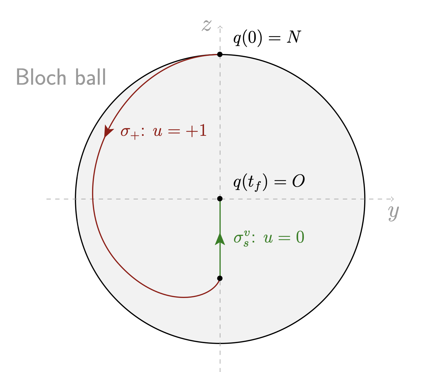
The time-minimal saturation problem is the following: starting from the North pole of the Bloch ball, the goal is to reach in minimum time the center of the Bloch ball, which corresponds at the final time to zero magnetization of the spin.

Time-minimal saturation problem

We define the time-minimal saturation problem as the following optimal control problem:

\[ \inf t_f, \quad \text{s.t.} \quad u(\cdot) \in \mathcal{U}, \quad t_f \ge 0 \quad \text{and} \quad q(t_f, N, u(\cdot)) = O,\]

where $N = (0, 1)$ is the North pole, where $O = (0,0)$ is the origin of the Bloch ball and where $t \mapsto q(t, q_0, u(\cdot))$ is the unique maximal solution of the 2D control system $\dot{q} = F_0(q) + u\, F_1(q)$ associated to the control $u(\cdot)$ and starting from the given initial condition $q_0$.

The inversion sequence ${\sigma_+} {\sigma_s^v}$, that is a positive bang arc followed by a singular vertical arc with zero control, is the simplest way to go from $N$ to $O$. Is it optimal?

We have the following symmetry.

Proposition. Let $(y(\cdot), z(\cdot))$, with associated control $u(\cdot)$, be a trajectory solution of $\dot{q} = F_0(q) + u\, F_1(q)$. Then, $(-y(\cdot), z(\cdot))$ with control $-u(\cdot)$ is also solution of this system.

This discrete symmetry allows us to consider only trajectories inside the domain $\{y \le 0\}$ of the Bloch ball.

In order to solve numerically the problem, we need to set the parameters. We introduce the practical cases in the following table. We give the relaxation times with the associated $(\gamma, \Gamma)$ parameters for $\omega_\mathrm{max} = 2 \pi\times 32.3$ Hz. Note that in the experiments, $\omega_\mathrm{max}$ may be chosen up to 15 000 Hz but we consider the same value as in ^[1].

Name	$T_1$	$T_2$	$\gamma$	$\Gamma$	$\delta=\gamma-\Gamma$
Water	2.5	2.5	$1.9710e^{-03}$	$1.9710e^{-03}$	$0.0$
Cerebrospinal Fluid	2.0	0.3	$2.4637e^{-03}$	$1.6425e^{-02}$	$-1.3961^{-02}$
Deoxygenated blood	1.35	0.05	$3.6499e^{-03}$	$9.8548e^{-02}$	$-9.4898^{-02}$
Oxygenated blood	1.35	0.2	$3.6499e^{-03}$	$2.4637e^{-02}$	$-2.0987^{-02}$
Gray cerebral matter	0.92	0.1	$5.3559e^{-03}$	$4.9274e^{-02}$	$-4.3918^{-02}$
White cerebral matter	0.78	0.09	$6.3172e^{-03}$	$5.4749e^{-02}$	$-4.8432^{-02}$
Fat	0.2	0.1	$2.4637e^{-02}$	$4.9274e^{-02}$	$-2.4637^{-02}$
Brain	1.062	0.052	$4.6397e^{-03}$	$9.4758e^{-02}$	$-9.0118^{-02}$
Parietal muscle	1.2	0.029	$4.1062e^{-03}$	$1.6991e^{-01}$	$-1.6580^{-02}$

Table: Matter name with associated relaxation times in seconds and relative $(\gamma, \Gamma)$ parameters with $\omega_\mathrm{max} = 2 \pi\times 32.3$ Hz and $u_\mathrm{max} = 1$.

Deoxygenated blood case

We consider the Deoxygenated blood case. According to Theorem 3.6 from ^[2] the optimal solution is of the form Bang-Singular-Bang-Singular (BSBS). The two bang arcs are with control $u=1$. The first singular arc is contained in the horizontal line $z=\gamma/2\delta$ while the second singular arc is contained in the vertical line $y=0$. We propose in the following to retrieve this result numerically.

Let us first define the parameters with the two vector fields $F_0$ and $F_1$.

import OptimalControl: ⋅
⋅(a::Number, b::Number) = a*b

# Blood case
T1 = 1.35 # s
T2 = 0.05

ω = 2π⋅32.3 # Hz
γ = 1/(ω⋅T1)
Γ = 1/(ω⋅T2)

δ = γ - Γ
zs = γ / 2δ # ordinate of the horizontal singular line

F0(y, z) = [-Γ⋅y, γ⋅(1-z)]
F1(y, z) = [-z, y]

q0 = [0, 1] # initial state: the North pole

Then, we can define the problem with OptimalControl.

using OptimalControl

ocp = @def begin

    tf ∈ R, variable
    t ∈ [0, tf ], time
    q = (y, z) ∈ R², state
    u ∈ R, control

    y(t) ≤ 0.1 # for the symmetry

    q(0)  == q0
    q(tf) == [0, 0]

    -1 ≤ u(t) ≤ 1

    q̇(t) == F0(q(t)...) + u(t) * F1(q(t)...)

    tf → min

    tf ≥ 0

end

Direct method

We start to solve the problem with a direct method. The problem is transcribed into a NLP optimization problem by OptimalControl. The NLP problem is then solved by the well-known solver Ipopt thanks to NLPModelsIpopt.

We first start with a coarse grid, with only 100 points. We provide an init consistent with a solution in the domain $y \le 0$.

using NLPModelsIpopt
N = 100
sol = solve(
    ocp;
    grid_size=N,
    init=(state=[-0.5, 0.0], ),
    disc_method=:gauss_legendre_2,
    print_level=4
)

▫ This is OptimalControl version v1.1.3 running with: direct, adnlp, ipopt.

▫ The optimal control problem is solved with CTDirect version v0.17.3.

   ┌─ The NLP is modelled with ADNLPModels and solved with NLPModelsIpopt.
   │
   ├─ Number of time steps⋅: 100
   └─ Discretisation scheme: gauss_legendre_2

Total number of variables............................:      703
                     variables with only lower bounds:        1
                variables with lower and upper bounds:      100
                     variables with only upper bounds:      101
Total number of equality constraints.................:      604
Total number of inequality constraints...............:        0
        inequality constraints with only lower bounds:        0
   inequality constraints with lower and upper bounds:        0
        inequality constraints with only upper bounds:        0


Number of Iterations....: 143

                                   (scaled)                 (unscaled)
Objective...............:   4.2714529345077786e+01    4.2714529345077786e+01
Dual infeasibility......:   7.2743894241611429e-13    7.2743894241611429e-13
Constraint violation....:   1.1102230246251565e-16    1.1102230246251565e-16
Variable bound violation:   9.9751860105357082e-09    9.9751860105357082e-09
Complementarity.........:   1.0000006641016691e-11    1.0000006641016691e-11
Overall NLP error.......:   1.0000006641016691e-11    1.0000006641016691e-11


Number of objective function evaluations             = 209
Number of objective gradient evaluations             = 133
Number of equality constraint evaluations            = 209
Number of inequality constraint evaluations          = 0
Number of equality constraint Jacobian evaluations   = 149
Number of inequality constraint Jacobian evaluations = 0
Number of Lagrangian Hessian evaluations             = 143
Total seconds in IPOPT                               = 4.903

EXIT: Optimal Solution Found.

Then, we plot the solution thanks to Plots.

using Plots
plt = plot(sol; size=(700, 500), label="N = "*string(N))

This rough approximation is then refine on a finer grid of 1000 points. This two steps resolution increases the speed of convergence. Note that we provide the previous solution as initialisation.

N = 1000
direct_sol = solve(
    ocp;
    grid_size=N,
    init=sol,
    disc_method=:gauss_legendre_2,
    print_level=4,
    tol=1e-12
)

▫ This is OptimalControl version v1.1.3 running with: direct, adnlp, ipopt.

▫ The optimal control problem is solved with CTDirect version v0.17.3.

   ┌─ The NLP is modelled with ADNLPModels and solved with NLPModelsIpopt.
   │
   ├─ Number of time steps⋅: 1000
   └─ Discretisation scheme: gauss_legendre_2

Total number of variables............................:     7003
                     variables with only lower bounds:        1
                variables with lower and upper bounds:     1000
                     variables with only upper bounds:     1001
Total number of equality constraints.................:     6004
Total number of inequality constraints...............:        0
        inequality constraints with only lower bounds:        0
   inequality constraints with lower and upper bounds:        0
        inequality constraints with only upper bounds:        0


Number of Iterations....: 55

                                   (scaled)                 (unscaled)
Objective...............:   4.2713711084173745e+01    4.2713711084173745e+01
Dual infeasibility......:   9.6456176379433600e-13    9.6456176379433600e-13
Constraint violation....:   2.7755575615628914e-16    2.7755575615628914e-16
Variable bound violation:   9.9883199489170238e-09    9.9883199489170238e-09
Complementarity.........:   5.0000406364690906e-13    5.0000406364690906e-13
Overall NLP error.......:   9.6456176379433600e-13    9.6456176379433600e-13


Number of objective function evaluations             = 79
Number of objective gradient evaluations             = 56
Number of equality constraint evaluations            = 79
Number of inequality constraint evaluations          = 0
Number of equality constraint Jacobian evaluations   = 57
Number of inequality constraint Jacobian evaluations = 0
Number of Lagrangian Hessian evaluations             = 55
Total seconds in IPOPT                               = 3.523

EXIT: Optimal Solution Found.

We can compare both solutions. The BSBS structure is revelead even if the second bang arc is not clearly demonstrated.

plot!(plt, direct_sol; label="N = "*string(N), color=2)

Code for plotting in the Bloch ball

We define a custom plot function for plotting the solution inside the Bloch ball.

Click to unfold and get the code of the custom plot function.

using Plots.PlotMeasures
function spin_plot(sol; kwargs...)

    y2 = cos(asin(zs))
    y1 = -y2

    t = time_grid(sol)
    q = state(sol)
    y = t -> q(t)[1]
    z = t -> q(t)[2]
    u = control(sol)

    # styles
    Bloch_ball_style = (seriestype=[:shape, ], color=:grey, linecolor=:black,
        legend=false, fillalpha=0.1, aspect_ratio=1)
    state_style = (label=:none, linewidth=2, color=1)
    initial_point_style = (seriestype=:scatter, color=:1, linewidth=0)
    axis_style = (color=:black, linewidth=0.5)
    control_style = (label=:none, linewidth=2, color=1)

    # state trajectory in the Bloch ball
    θ = LinRange(0, 2π, 100)
    state_plt = plot(cos.(θ), sin.(θ); Bloch_ball_style...) # Bloch ball
    plot!(state_plt, [-1, 1], [ 0,  0]; axis_style...)      # horizontal axis
    plot!(state_plt, [ 0, 0], [-1,  1]; axis_style...)      # vertical axis
    plot!(state_plt, [y1, y2], [zs, zs]; linestyle=:dash, axis_style...) # singular line
    plot!(state_plt, y.(t), z.(t); state_style...)
    plot!(state_plt, [0], [1]; initial_point_style...)
    plot!(state_plt; xlims=(-1.1, 0.1), ylims=(-0.1, 1.1), xlabel="y", ylabel="z")

    # control
    control_plt = plot(legend=false)
    plot!(control_plt, [ 0, t[end]], [1,  1]; linestyle=:dash, axis_style...) # upper bound
    plot!(control_plt, [ 0, t[end]], [0,  0]; linestyle=:dash, axis_style...)
    plot!(control_plt, [ 0, 0], [-0.1,  1.1]; axis_style...)
    plot!(control_plt, [ t[end], t[end]], [-0.1,  1.1]; axis_style...)
    plot!(control_plt, t, u.(t); control_style...)
    plot!(control_plt; ylims=(-0.1, 1.1), xlabel="t", ylabel="u")

    return plot(state_plt, control_plt; layout=(1, 2), leftmargin=15px, bottommargin=15px, kwargs...)

end

Below, we plot the solution inside the Bloch ball. The first bang arc drives the trajectory to the horizontal singular line $z = \gamma / (2\delta)$, shown as a dashed line. The second bang arc is very short, which makes it difficult to capture accurately unless the grid is sufficiently fine. In the next section, we introduce an indirect method to refine this approximation.

spin_plot(direct_sol; size=(800, 400))

To make the indirect method converge we need a good initial guess. We extract below the useful information from the direct solution to provide an initial guess for the indirect method. We need the initial costate together with the switching times between bang and singular arcs and the final time.

t  = time_grid(direct_sol)
q  = state(direct_sol)
p  = costate(direct_sol)
u  = control(direct_sol)
tf = variable(direct_sol)

t0 = 0
pz0 = p(t0)[2]

t_bang_1 = t[ (abs.(u.(t)) .≥ 0.5) .& (t .≤  5)]
t_bang_2 = t[ (abs.(u.(t)) .≥ 0.5) .& (t .≥ 35)]
t1 = max(t_bang_1...)
t2 = min(t_bang_2...)
t3 = max(t_bang_2...)

q1, p1 = q(t1), p(t1)
q2, p2 = q(t2), p(t2)
q3, p3 = q(t3), p(t3)

println("pz0 = ", pz0)
println("t1 = ", t1)
println("t2 = ", t2)
println("t3 = ", t3)
println("tf = ", tf)

pz0 = -10.138145104720211
t1 = 1.6231210211986022
t2 = 37.118214932146984
t3 = 37.545352042988725
tf = 42.713711084173745

Indirect method

We introduce the pseudo-Hamiltonian

\[H(q, p, u) = H_0(q, p) + u\, H_1(q, p)\]

where $H_0(q, p) = p \cdot F_0(q)$ and $H_1(q, p) = p \cdot F_1(q)$ are both Hamiltonian lifts. According to the maximisation condition from the Pontryagin Maximum Principle (PMP), a bang arc occurs when $H_1$ is nonzero and of constant sign along the arc. On the contrary the singular arcs are contained in $H_1 = 0$. If $t \mapsto H_1(q(t), p(t)) = 0$ along an arc then its derivative is also zero. Thus, along a singular arc we have also

\[\frac{\mathrm{d}}{\mathrm{d}t} H_1(q(t), p(t)) = \{H_0, H_1\}(q(t), p(t)) = 0,\]

where $\{H_0, H_1\}$ is the Poisson bracket of $H_0$ and $H_1$.

Lie and Poisson brackets

Let $F_0$, $F_1$ be two smooth vector fields on a smooth manifold $M$ and $f$ a smooth function on $M$. Let $x$ be local coordinates. The Lie bracket of $F_0$ and $F_1$ is given by

\[ [F_0,F_1] \coloneqq F_0 \cdot F_1 - F_1 \cdot F_0,\]

with $(F_0 \cdot F_1)(x) = \mathrm{d} F_1(x) \cdot F_0(x)$. The Lie derivative $\mathcal{L}_{F_0} f$ of $f$ along $F_0$ is simply written $F_0\cdot f$. Denoting $H_0$, $H_1$ the Hamiltonian lifts of $F_0$, $F_1$, then the Poisson bracket of $H_0$ and $H_1$ is

\[ \{H_0,H_1\} \coloneqq \vec{H_0} \cdot H_1.\]

We also use the notation $H_{01}$ (resp. $F_{01}$) to write the bracket $\{H_0,H_1\}$ (resp. $[F_0,F_1]$) and so forth. Besides, since $H_0$, $H_1$ are Hamiltonian lifts, we have $\{H_0,H_1\}= p \cdot [F_0,F_1]$.

Code for plotting the switching function and its derivative

We define a function for plotting the switching function $t \mapsto H_1(q(t), p(t))$ and its derivative along the solution computed by the direct method.

Click to unfold and get the code of the function.

function switching_plot(sol, H1, H01; kwargs...)

    t  = time_grid(sol)
    u  = control(sol)
    q  = state(sol)
    p  = costate(sol)
    tf = t[end]
    φ(t) = H1(q(t), p(t))       # switching function
    dφ(t) = H01(q(t), p(t))     # derivative of the switching function

    # styles
    axis_style = (color=:black, linewidth=0.5, label=false)
    control_style = (label=:none, linewidth=2, color=1)

    # switching function
    switching_plt = plot()
    plot!(switching_plt, [0, tf], [0, 0]; axis_style...)
    plot!(switching_plt, t, φ, label="H1(q(t), p(t))", xlabel="t", linewidth=2)
    plot!(switching_plt; xlims=(0, tf))

    # derivative of the switching function
    dswitching_plt = plot()
    plot!(dswitching_plt, [0, tf], [0, 0]; axis_style...)
    plot!(dswitching_plt, t, dφ, label="H01(q(t), p(t))", xlabel="t", linewidth=2)
    plot!(dswitching_plt; xlims=(0, tf))

    # control
    control_plt = plot(legend=false)
    plot!(control_plt, [ 0, t[end]], [1,  1]; linestyle=:dash, axis_style...) # upper bound
    plot!(control_plt, [ 0, t[end]], [0,  0]; linestyle=:dash, axis_style...)
    plot!(control_plt, [ 0, 0], [-0.1,  1.1]; axis_style...)
    plot!(control_plt, [ t[end], t[end]], [-0.1,  1.1]; axis_style...)
    plot!(control_plt, t, u.(t); control_style...)
    plot!(control_plt; ylims=(-0.1, 1.1), xlabel="t", ylabel="u")

    return plot(switching_plt, dswitching_plt, control_plt; layout=(3, 1), kwargs...)
end

We can notice on the plots below that maximisation condition from the PMP is not satisfied. We can see that the switching function becomes negative along the first bang arc but there is no switching from the control plot. Besides, we can see that along the first singular arc, the switching function is not always zero.

H0 = Lift(q -> F0(q...))
H1 = Lift(q -> F1(q...))
H01  = @Lie { H0, H1 }

switching_plot(direct_sol, H1, H01; size=(700, 800))

We aim to compute a better approximation of the solution thanks to indirect shooting. To do so, we need to define the three different flows associated to the three different control laws in feedback form: bang control, singular control along the horizontal line and singular control along the vertical line.

Note

Let us recall that $\delta = \gamma - \Gamma$. Then, for any $q = (y,z)$ we have:

\[ \begin{aligned} F_{01}(q) &= -(\gamma - \delta z) \frac{\partial}{\partial y} + \delta y \frac{\partial}{\partial z}, \\[0.5em] F_{001}(q) &= \left( \gamma\, (\gamma - 2\Gamma) - \delta^2 z\right)\frac{\partial}{ \partial y} + \delta^2 y \frac{\partial}{\partial z}, \\[0.5em] F_{101}(q) &= 2 \delta y \frac{\partial}{\partial y} + (\gamma - 2 \delta z) \frac{\partial}{\partial z}. \end{aligned}\]

Along a singular arc, we have $H_1 = H_{01} = 0$, that is $p \cdot F_1 = p \cdot F_{01} = 0$. Since, $p$ is of dimension 2 and is nonzero, then we have $\det(F_1, F_{01}) = y ( \gamma - 2 \delta z) = 0$. This gives us the two singular lines.

Differentiating $t \mapsto H_1(q(t), p(t)) = 0$ a second time along a singular arc gives

\[ H_{001}(q(t), p(t)) + u(t)\, H_{101}(q(t), p(t)) = 0,\]

that is $p(t)$ is orthogonal to $F_{001}(q(t)) + u(t)\, F_{101}(q(t))$. Hence, the singular control is given by

\[ \det(F_1(q(t)), F_{001}(q(t))) + u(t) \, \det(F_1(q(t)), F_{101}(q(t))) = 0.\]

For $y=0$, $\det(F_1(q), F_{101}(q))$ is zero and thus the singular control is zero. We denote it $u_0 \coloneqq 0$. Along the horizontal singular line, that is for $z=\gamma/2\delta$, the control is given by

\[ u_s(y) \coloneqq \gamma (2\Gamma - \gamma) / (2 \delta y).\]

Note that we could have defined the singular control with the Hamiltonian lifts $H_{001}$ and $H_{101}$. See the Goddard tutorial for an example of such a computation.

using OrdinaryDiffEq

# Controls
u0 = 0                   # off control: vertical singular line
u1 = 1                   # positive bang control
us(y) = γ⋅(2Γ−γ)/(2δ⋅y)  # singular control: horizontal line

# Flows
options = (abstol=1e-14, reltol=1e-10)

f0 = Flow(ocp, (q, p, tf) -> u0      ; options...)
f1 = Flow(ocp, (q, p, tf) -> u1      ; options...)
fs = Flow(ocp, (q, p, tf) -> us(q[1]); options...)

With the previous flows, we can define the shooting function considering the sequence given by the direct method: Bang-Singular-Bang-Singular. There are 3 switching times $t_1$, $t_2$ and $t_3$. The final time $t_f$ is unknown such as the initial costate. To reduce the sensitivy of the shooting function we also consider the states and costates at the switching times as unknowns and we add some matching conditions.

Note that the final time is free, hence, in the normal case, $H = -p^0 = 1$ along the solution of the PMP. Considering this condition at the initial time ($H$ is constant since the system is autonomous), we obtain $p_y(0) = -1$. At the entrance of the singular arcs, we must satisfy $H_1 = H_{01} = 0$. For the first singular arc, this leads to the conditions

\[ - p_y(t_1) z_s + p_z(t_1) y(t_1) = z(t_1) - z_s = 0.\]

At the entrance of the second singular arc, we have

\[ p_y(t_3) = y(t_3) = 0.\]

Finally, the solution has to satisfy the final condition $q(t_f) = (y(t_f), z(t_f)) = (0, 0)$. Since, the last singular arc is contained in $y=0$, the condition $y(t_f)=0$ is redundant and so we only need to check that $z(t_f) = 0$.

Altogether, this leads to the following shooting function.

function shoot!(s, pz0, t1, t2, t3, tf, q1, p1, q2, p2, q3, p3)

    p0 = [-1, pz0]

    q1_, p1_ = f1(t0, q0, p0, t1)
    q2_, p2_ = fs(t1, q1, p1, t2)
    q3_, p3_ = f1(t2, q2, p2, t3)
    qf , pf  = f0(t3, q3, p3, tf)

    s[1] = - p1[1] ⋅ zs + p1[2] ⋅ q1[1]   # H1 = H01 = 0 on the horizontal
    s[2] = q1[2] - zs                     # singular line, z=zs
    s[3] = p3[1]                          # H1 = H01 = 0 on the vertical
    s[4] = q3[1]                          # singular line, y=0
    s[5] = qf[2]                          # z(tf) = 0

    # matching conditions
    s[ 6: 7] = q1 - q1_
    s[ 8: 9] = p1 - p1_
    s[10:11] = q2 - q2_
    s[12:13] = p2 - p2_
    s[14:15] = q3 - q3_
    s[16:17] = p3 - p3_

end

We are now in position to solve the shooting equations. Due to the sensitivity of the first singular arc, we need to improve the initial guess obtained from the direct method to make the Newton solver converge. To do so, we set for the initial guess $z(t_1) = z_s$ and $p_z(t_1) = p_y(t_1) z_s / y(t_1)$.

We can see below from the norm of the shooting function that the initial guess is not very accurate.

# we refine the initial guess to make the Newton solver converge
q1[2] = zs
p1[2] = p1[1] ⋅ zs / q1[1]

# Norm of the shooting function at initial guess
using LinearAlgebra: norm

s = similar([pz0], 17)
shoot!(s, pz0, t1, t2, t3, tf, q1, p1, q2, p2, q3, p3)

println("Norm of the shooting function: ‖s‖ = ", norm(s), "\n")

Norm of the shooting function: ‖s‖ = 18.361555100489344

We can use the MINPACK.jl package to solve the shooting equation. To compute the Jacobian of the shooting function we use the DifferentiationInterface.jl package with ForwardDiff.jl backend.

using DifferentiationInterface
import ForwardDiff
backend = AutoForwardDiff()

Let us define the problem to solve.

# auxiliary function with aggregated inputs
shoot!(s, ξ) = shoot!(s, ξ[1], ξ[2:5]..., ξ[6:7], ξ[8:9],
    ξ[10:11], ξ[12:13], ξ[14:15], ξ[16:17])

# Jacobian of the (auxiliary) shooting function
jshoot!(js, ξ) = jacobian!(shoot!, similar(ξ), js, backend, ξ)

We are now in position to solve the problem with the hybrj solver from MINPACK.jl through the fsolve function, providing the Jacobian. Let us solve the problem and retrieve the initial contate and the times (switching and final) from the solution.

using MINPACK

# initial guess
ξ = [ pz0 ; t1 ; t2 ; t3 ; tf ; q1 ; p1 ; q2 ; p2 ; q3 ; p3]

# resolution of S(ξ) = 0
indirect_sol = fsolve(shoot!, jshoot!, ξ, show_trace=true)

# we retrieve the costate solution together with the times
pz0 = indirect_sol.x[1]
t1 = indirect_sol.x[2]
t2 = indirect_sol.x[3]
t3 = indirect_sol.x[4]
tf = indirect_sol.x[5]
q1 = indirect_sol.x[6:7]
p1 = indirect_sol.x[8:9]
q2 = indirect_sol.x[10:11]
p2 = indirect_sol.x[12:13]
q3 = indirect_sol.x[14:15]
p3 = indirect_sol.x[16:17]

println("pz0 = ", pz0)
println("t1 = ", t1)
println("t2 = ", t2)
println("t3 = ", t3)
println("tf = ", tf)

# Norm of the shooting function at solution
s = similar([pz0], 17)
shoot!(s, pz0, t1, t2, t3, tf, q1, p1, q2, p2, q3, p3)
println("Norm of the shooting function: ‖s‖ = ", norm(s), "\n")

Iter     f(x) inf-norm    Step 2-norm      Step time
------   --------------   --------------   --------------
     1     1.729122e+01     0.000000e+00         0.233449
     2     9.461468e-01     3.704268e+01        31.985831
     3     2.839417e-01     7.649105e+00         0.004164
     4     2.196746e-01     6.189414e+00         0.004116
     5     4.899687e-02     1.555075e+01         0.004046
     6     1.317601e-01     6.220299e+01         0.003931
     7     3.647552e-01     1.399561e+02         0.004005
     8     4.266673e-02     3.889313e+00         0.052066
     9     1.862372e-01     1.555075e+01         0.004261
    10     3.906691e-02     3.889347e+00         0.004261
    11     6.814071e-02     3.887687e+00         0.004280
    12     1.408918e-02     9.722099e-01         0.004234
    13     4.460910e-02     3.887687e+00         0.004350
    14     9.719317e-03     9.720021e-01         0.004358
    15     4.894523e-02     3.887687e+00         0.004342
    16     1.037975e-02     9.720452e-01         0.004248
    17     1.722110e-02     9.719218e-01         0.004340
    18     3.374491e-03     2.429959e-01         0.004450
    19     1.050803e-02     9.719218e-01         0.004301
    20     2.514214e-03     2.429847e-01         0.004338
    21     1.236260e-02     9.719218e-01         0.005304
    22     2.699892e-03     2.429877e-01         0.006105
    23     4.405108e-03     2.429804e-01         0.006158
    24     1.140801e-03     6.074605e-02         0.006111
    25     2.529561e-03     2.429804e-01         0.006108
    26     8.971382e-04     6.074537e-02         0.018664
    27     3.105367e-03     2.429804e-01         0.004269
    28     6.886897e-04     6.074555e-02         0.004252
    29     1.114999e-03     6.074511e-02         0.004191
    30     5.937321e-04     1.518634e-02         0.004264
    31     6.886842e-04     6.074511e-02         0.004174
    32     5.243157e-04     1.518629e-02         0.004152
    33     7.780883e-04     6.074511e-02         0.004239
    34     4.570424e-04     1.518630e-02         0.004220
    35     7.861590e-04     6.074511e-02         0.004350
    36     3.925009e-04     1.518631e-02         0.004208
    37     7.834904e-04     6.074511e-02         0.004203
    38     3.308893e-04     1.518631e-02         0.004264
    39     7.850448e-04     6.074511e-02         0.004959
    40     2.723456e-04     1.518631e-02         0.014794
    41     7.867550e-04     6.074511e-02         0.004267
    42     2.170459e-04     1.518631e-02         0.004313
    43     7.883592e-04     6.074511e-02         0.004269
    44     1.793299e-04     1.518631e-02         0.004309
    45     7.899762e-04     6.074511e-02         0.004288
    46     1.787759e-04     1.518631e-02         0.004432
    47     2.839177e-04     1.518628e-02         0.004357
    48     1.589777e-04     3.796573e-03         0.004239
    49     1.503008e-04     1.518628e-02         0.004242
    50     1.506639e-04     3.796570e-03         0.004298
    51     1.968768e-04     1.518628e-02         0.004422
    52     1.424838e-04     3.796571e-03         0.012582
    53     1.995271e-04     1.518628e-02         0.004280
    54     1.342526e-04     3.796571e-03         0.004198
    55     1.981819e-04     1.518628e-02         0.004169
    56     1.259569e-04     3.796571e-03         0.004148
    57     1.983571e-04     1.518628e-02         0.004130
    58     1.175940e-04     3.796571e-03         0.004129
    59     1.986120e-04     1.518628e-02         0.004161
    60     1.091543e-04     3.796571e-03         0.004136
    61     1.988165e-04     1.518628e-02         0.004195
    62     1.006264e-04     3.796571e-03         0.004279
    63     1.990215e-04     1.518628e-02         0.010366
    64     9.199662e-05     3.796571e-03         0.004290
    65     7.942206e-05     3.796569e-03         0.004319
    66     8.723076e-05     9.491426e-04         0.004263
    67     7.506890e-05     3.796569e-03         0.004299
    68     1.671472e-04     1.518628e-02         0.004259
    69     6.666613e-05     3.796571e-03         0.004321
    70     6.134117e-05     9.491423e-04         0.026285
    71     4.993157e-05     3.796569e-03         0.004174
    72     5.647322e-05     9.491424e-04         0.004176
    73     4.774480e-05     3.796569e-03         0.004126
    74     5.160141e-05     9.491424e-04         0.004114
    75     4.774434e-05     3.796569e-03         0.004112
    76     4.672440e-05     9.491424e-04         0.004152
    77     4.776050e-05     3.796569e-03         0.009522
    78     4.183995e-05     9.491424e-04         0.004266
    79     4.777701e-05     3.796569e-03         0.004302
    80     3.694530e-05     9.491424e-04         0.004293
    81     4.779395e-05     3.796569e-03         0.004319
    82     3.203693e-05     9.491424e-04         0.004257
    83     4.781139e-05     3.796569e-03         0.004444
    84     2.711018e-05     9.491424e-04         0.004400
    85     4.782921e-05     3.796569e-03         0.004242
    86     2.215861e-05     9.491424e-04         0.004233
    87     4.784746e-05     3.796569e-03         0.004308
    88     1.717278e-05     9.491424e-04         0.012668
    89     4.786615e-05     3.796569e-03         0.004261
    90     1.213745e-05     9.491424e-04         0.004166
    91     4.788530e-05     3.796569e-03         0.004184
    92     8.099735e-06     9.491424e-04         0.004134
    93     2.324557e-05     1.548720e-03         0.004149
    94     2.321026e-06     7.302771e-05         0.004125
    95     2.874311e-06     7.491454e-05         0.004165
    96     1.820909e-08     1.764393e-10         0.004188
    97     4.602427e-09     9.546174e-12         0.004175
    98     2.378469e-12     3.583026e-13         0.004265
pz0 = -10.103027162172843
t1 = 1.6450509469600776
t2 = 37.323981285581745
t3 = 37.58077357861729
tf = 42.71370875363171
Norm of the shooting function: ‖s‖ = 2.6791056126541833e-12

Let us plot the solution from the indirect method. We can notice that the second bang arc is well captured by the indirect method compared to the direct method.

# concatenation of the flows with the switching times
f = f1 * (t1, fs) * (t2, f1) * (t3, f0)

# computation of the solution: state, costate, control
indirect_sol = f((t0, tf), q0, [-1, pz0])

# plot in the Bloch ball
spin_plot(indirect_sol; size=(800, 400))

From the following plot, we can conclude that the maximisation condition from the PMP is now well satisfied compared to the solution obtained from the direct method.

plt = switching_plot(indirect_sol, H1, H01; size=(700, 800))
lens!(plt, [37.2, 37.7], [    0, 4e-5], inset = (1, bbox(0.3, 0.2, 0.3, 0.4)))
lens!(plt, [37.2, 37.7], [-5e-4, 5e-4], inset = (2, bbox(0.3, 0.3, 0.3, 0.4)))
lens!(plt, [37.2, 37.7], [  0.5,  1.1], inset = (3, bbox(0.3, 0.2, 0.3, 0.4)))

1B. Bonnard, O. Cots, S. Glaser, M. Lapert, D. Sugny & Y. Zhang, *Geometric optimal control of the contrast imaging problem in nuclear magnetic resonance, IEEE Trans. Automat. Control, 57 (2012), no. 8, 1957–1969.
2Bonnard, B.; Cots, O.; Rouot, J.; Verron, T. Time minimal saturation of a pair of spins and application in magnetic resonance imaging. Mathematical Control and Related Fields, 2020, 10 (1), pp.47-88. https://inria.hal.science/hal-01779377