OptimalControl.jl — a guided tour
This tutorial is a guided tour of OptimalControl.jl, part of the control-toolbox ecosystem. We follow two problems end to end: a simple double integrator for modelling, initialisation and the indirect (Pontryagin) method, and the Goddard rocket for the direct method in depth, grid continuation and GPU solving. Advanced topics are linked at the end.
It is written for readers with a background in optimal control, ODEs or optimisation. By the end you will be able to define an optimal control problem, solve it by both the direct and indirect methods, and visualise the result — all in a few lines of code.
You can run this tutorial interactively in your browser — no installation required — by clicking the Binder badge below:

The problem, and installing the tools
An optimal control problem (OCP) in Bolza form reads
\[J(x, u) = g(x(t_0), x(t_f)) + \int_{t_0}^{t_f} f^{0}(t, x(t), u(t))\,\mathrm{d}t \;\to\; \min,\]
subject to the controlled dynamics $\dot{x}(t) = f(t, x(t), u(t))$ and, possibly, box / path / boundary constraints. When $g = 0$ the cost is of Lagrange form; when $f^0 = 0$, of Mayer form.
More generally, the times $t_0$ and $t_f$ may be free (optimisation variables), and a vector $v$ of additional parameters can enter the cost, dynamics and constraints. The full problem then reads
\[\min_{x,u,v}\; g(x(t_0), x(t_f), v) + \int_{t_0}^{t_f} f^{0}(t, x(t), u(t), v)\,\mathrm{d}t,\]
subject to $\dot{x}(t) = f(t, x(t), u(t), v)$, box / path / boundary constraints.
OptimalControl.jl is the core of the control-toolbox ecosystem, a modular suite of Julia packages — CTBase (base types & exceptions), CTParser (DSL parsing), CTModels (problem data structures), CTDirect (discretisation & NLP transcription), CTFlows (Hamiltonian flows for indirect methods), and CTSolvers (solver orchestration) — that can also be used individually.
Installation is a single package:
import Pkg
Pkg.add("OptimalControl")
We load OptimalControl.jl to model the problem, a solver backend (NLPModelsIpopt.jl), and Plots.jl.
using OptimalControl
using NLPModelsIpopt
using Plots
Defining a problem: @def vs macro-free
Our running example: a wagon of unit mass on a frictionless rail, state $x = (q, v)$ (position, velocity), acceleration controlled by a force $u$. We start at $(-1, 0)$, must reach $(0, 0)$ at $t_f = 1$, and minimise the transfer energy
\[\frac{1}{2}\int_0^1 u^2(t)\,\mathrm{d}t,\]
subject to the dynamics
\[\dot{q}(t) = v(t), \qquad \dot{v}(t) = u(t).\]
t0 = 0; tf = 1; x0 = [-1, 0]; xf = [0, 0];The @def macro
The @def macro lets us write the problem almost exactly as the mathematics:
Each line of the @def block mirrors a piece of the mathematical formulation — time, state, control, dynamics, boundary conditions, then cost — in the same order one would write them on paper. Unicode symbols (∈, R², ẋ, ∫, →) make the code read like the maths; plain ASCII alternatives (R^2, derivative, integral, =>) are available for keyboards or workflows that prefer them.
ocp = @def begin
    t ∈ [t0, tf], time
    x = (q, v) ∈ R², state
    u ∈ R, control

    x(t0) == x0
    x(tf) == xf

    ẋ(t) == [v(t), u(t)]

    0.5∫( u(t)^2 ) → min
end
The same problem with the macro-free (functional) API
The functional API builds the same model step by step with plain functions — useful for programmatic problem generation or macro-free library code.
pre = OptimalControl.PreModel()

time!(pre; t0=t0, tf=tf)
state!(pre, 2, "x", ["q", "v"])
control!(pre, 1)

function f_energy!(dx, t, x, u, v)
    dx[1] = x[2]
    dx[2] = u[1]
    return nothing
end
dynamics!(pre, f_energy!)

function boundary_energy!(b, x0_, xf_, v)
    b[1] = x0_[1] - x0[1]
    b[2] = x0_[2] - x0[2]
    b[3] = xf_[1] - xf[1]
    b[4] = xf_[2] - xf[2]
    return nothing
end
constraint!(pre, :boundary; f=boundary_energy!, lb=zeros(4), ub=zeros(4), label=:endpoint)

lagrange_energy(t, x, u, v) = 0.5 * u[1]^2
objective!(pre, :min; lagrange=lagrange_energy)

time_dependence!(pre; autonomous=true)

ocp_func = build(pre)
What the macro actually does
Key message: @def translates the expression into the very same functional calls, and additionally records the symbolic definition. We can see the difference directly: the macro keeps the DSL expression, whereas the functional API stores an empty definition.
definition(ocp) # the macro records the full DSL expressionAbstract definition:
t ∈ [t0, tf], time
x = ((q, v) ∈ R², state)
u ∈ R, control
x(t0) == x0
x(tf) == xf
ẋ(t) == [v(t), u(t)]
0.5 * ∫(u(t) ^ 2) → min
has_abstract_definition(ocp_func) # false: functional API stores no abstract definitionfalse- In the functional API, callbacks are always vector-valued: even when the control is scalar, one writes
u[1]— notu— insidef_energy!orlagrange_energy. - The functional API currently works only with the
:adnlpmodeler; it does not support the:examodeler needed for GPU solving — one more reason to prefer@defwhen GPU execution is contemplated (more in the GPU section).
First solve, initial guess, and the costate
Solving is one call, plotting another.
direct_sol = solve(ocp)▫ This is OptimalControl 2.0.4, solving with: collocation → adnlp → ipopt (cpu)
📦 Configuration:
├─ Discretizer: collocation
├─ Modeler: adnlp
└─ Solver: ipopt
▫ This is Ipopt version 3.14.19, running with linear solver MUMPS 5.8.2.
Number of nonzeros in equality constraint Jacobian...: 1754
Number of nonzeros in inequality constraint Jacobian.: 0
Number of nonzeros in Lagrangian Hessian.............: 250
Total number of variables............................: 752
variables with only lower bounds: 0
variables with lower and upper bounds: 0
variables with only upper bounds: 0
Total number of equality constraints.................: 504
Total number of inequality constraints...............: 0
inequality constraints with only lower bounds: 0
inequality constraints with lower and upper bounds: 0
inequality constraints with only upper bounds: 0
iter objective inf_pr inf_du lg(mu) ||d|| lg(rg) alpha_du alpha_pr ls
0 5.0000000e-03 1.10e+00 2.24e-14 0.0 0.00e+00 - 0.00e+00 0.00e+00 0
1 6.0000960e+00 2.22e-16 1.78e-15 -11.0 6.08e+00 - 1.00e+00 1.00e+00h 1
Number of Iterations....: 1
(scaled) (unscaled)
Objective...............: 6.0000960015360381e+00 6.0000960015360381e+00
Dual infeasibility......: 1.7763568394002505e-15 1.7763568394002505e-15
Constraint violation....: 2.2204460492503131e-16 2.2204460492503131e-16
Variable bound violation: 0.0000000000000000e+00 0.0000000000000000e+00
Complementarity.........: 0.0000000000000000e+00 0.0000000000000000e+00
Overall NLP error.......: 1.7763568394002505e-15 1.7763568394002505e-15
Number of objective function evaluations = 2
Number of objective gradient evaluations = 2
Number of equality constraint evaluations = 2
Number of inequality constraint evaluations = 0
Number of equality constraint Jacobian evaluations = 2
Number of inequality constraint Jacobian evaluations = 0
Number of Lagrangian Hessian evaluations = 1
Total seconds in IPOPT = 3.693
EXIT: Optimal Solution Found.• Solver:
✓ Successful : true
│ Status : first_order
│ Message : Ipopt/generic
│ Iterations : 1
│ Objective : 6.000096001536038
└─ Constraints violation : 2.220446049250313e-16
• Boundary duals: [12.000192003072058, 6.0000960015360265, -12.000192003072058, 6.000096001536031]
plot(direct_sol; size=(800, 600))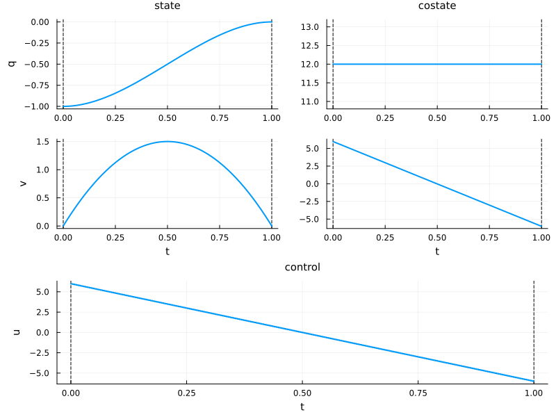
The default initial guess
With no initial guess, every variable is initialised to 0.1. We can see the initial guess without optimising, by stopping the solver immediately with max_iter=0:
sol_init = solve(ocp; init=nothing, max_iter=0, display=false)
plot(sol_init; size=(800, 600))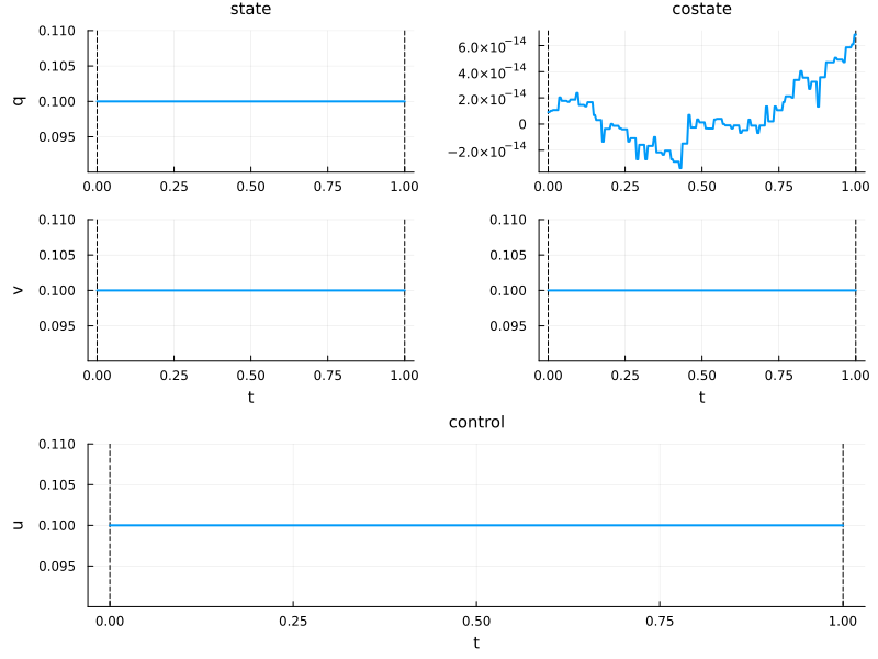
Even though we only ever provide the state, control and (optional) variable, the solver initialises the adjoint internally. After optimisation, this right-column costate is exactly the adjoint $p$ of Pontryagin's Maximum Principle — the same $p$ we will reuse to start the indirect method in the indirect section. This closes the loop between the direct and indirect methods.
Providing our own initial guess
The recommended way to provide an initial guess is the @init macro, using the labels from the @def block (q, v, u here):
ig = @init ocp begin
    q(t) := -1 + t
    v(t) := 0
    u(t) := 0
end

sol = solve(ocp; init=ig, display=false)
println("iterations, default guess: ", iterations(direct_sol))
println("iterations, @init guess:   ", iterations(sol))
iterations, default guess: 1
iterations, @init guess: 1In this case both guesses give 1 iteration: the double integrator is a linear-quadratic problem, so the NLP is quadratic and Ipopt solves it in a single step regardless of the starting point. Warm-starting only pays off on genuinely nonlinear problems — we will see this with the Goddard rocket in the next section.
For all the ways to specify an initial guess, see Set an initial guess.
There is currently no way to initialise the costate directly — only state, control and variable can be provided through @init. The solver initialises the adjoint internally (as we saw above). Costate initialisation is a planned feature.
Direct method in depth: Goddard
Discretise optimal control problems
The direct method turns the infinite-dimensional OCP into a finite-dimensional nonlinear program (NLP) by discretising time (Runge–Kutta / collocation) on a grid, then hands the NLP to a solver. It is robust and easy to use.
Concretely, time is discretised on a uniform grid $t_0 < t_1 < \dots < t_N = t_f$ with step $h = (t_f - t_0)/N$. The (explicit) Euler scheme, for instance, replaces the dynamics by
\[x_{i} = x_{i-1} + h\,f(t_{i-1}, x_{i-1}, u_{i-1}), \quad i = 1, \dots, N,\]
and the integral cost by the corresponding rectangle sum
\[h\sum_{i=0}^{N-1} f^{0}(t_i, x_i, u_i).\]
The continuous OCP thus becomes a finite-dimensional NLP in the variables $X = (x_0, \dots, x_N, u_0, \dots, u_N)$, which is passed to an NLP solver such as Ipopt. Higher-order schemes (midpoint, Gauss–Legendre collocation) follow the same principle with different quadrature and interpolation formulas — solve defaults to the second-order :midpoint scheme, not Euler.
The Goddard rocket problem
To demonstrate convergence behaviour and warm-starting, we need a genuinely nonlinear problem. The Goddard rocket — maximise the final altitude, with free final time and a singular arc — is a classic test case.
# Goddard data and dynamics (F0: drift, F1: thrust)
const r0 = 1
const v0 = 0
const m0 = 1
const mf = 0.6
const Cd = 310
const Tmax = 3.5
const β = 500
const b = 2

F0(x) = begin
    r, v, m = x
    D = Cd * v^2 * exp(-β * (r - 1))
    [v, -D/m - 1/r^2, 0]
end
F1(x) = begin
    r, v, m = x
    [0, Tmax/m, -b*Tmax]
end

goddard = @def begin
    tf ∈ R, variable
    t ∈ [t0, tf], time
    x = (r, v, m) ∈ R³, state
    u ∈ R, control

    x(t0) == [r0, v0, m0]
    m(tf) == mf
    0 ≤ u(t) ≤ 1
    r(t) ≥ r0

    ẋ(t) == F0(x(t)) + u(t) * F1(x(t))

    r(tf) → max
end
Choosing a solver is trivial
solve uses the defaults (collocation, ADNLP modeler, Ipopt, CPU). Switching solver is just loading a package and passing a token (see Solve a problem):
using MadNLP

sol_ipopt  = solve(goddard;          grid_size=250, display=false)
sol_madnlp = solve(goddard, :madnlp; grid_size=250, display=false)

println("Ipopt  : r(tf) = ", objective(sol_ipopt),  ", ", iterations(sol_ipopt),  " iters")
println("MadNLP : r(tf) = ", objective(sol_madnlp), ", ", iterations(sol_madnlp), " iters")
Ipopt : r(tf) = 1.0128374184916846, 95 iters
MadNLP : r(tf) = 1.0128372815654052, 28 itersThe available methods and their options can be inspected with methods() and describe(:collocation); we will not dwell on them here.
Grid continuation by warm-starting
A solution can be passed directly as the initial guess of another solve — it is interpolated onto the new grid. This makes discrete continuation trivial and ties back to the initialisation above. On this nonlinear problem it genuinely pays: we compare reaching a fine grid of 1000 two ways:
- cold start — solve
grid_size=1000directly; - cascade — solve
grid_size=50first, thengrid_size=1000warm-started with that solution.
# solutions computed once, reused for iteration counts and the overlay plot
sol_cold = solve(goddard; grid_size=1000, display=false)

# warm cascade: grid 50 first, then grid 1000 initialised from it
s50   = solve(goddard; grid_size=50, display=false)
s1000 = solve(goddard; grid_size=1000, init=s50, display=false)

println("cold    grid 1000        : ", iterations(sol_cold), " iters")
println("cascade grid 50 (warm-up): ", iterations(s50),      " iters")
println("cascade grid 1000 (warm) : ", iterations(s1000),    " iters")
cold grid 1000 : 186 iters
cascade grid 50 (warm-up): 57 iters
cascade grid 1000 (warm) : 13 itersMessage: what matters is the iteration count at the expensive grid — the warm-started iterations(s1000) is well below the cold iterations(sol_cold), even though the cheap grid_size=50 warm-up adds iterations of its own to the running total; since a grid-50 iteration is far cheaper than a grid-1000 iteration, the cascade still wins on wall-clock time. Overlay the successive solutions to watch convergence:
plt = plot(s50;  label="50", size=(800, 800))
plot!(plt, s1000; label="1000")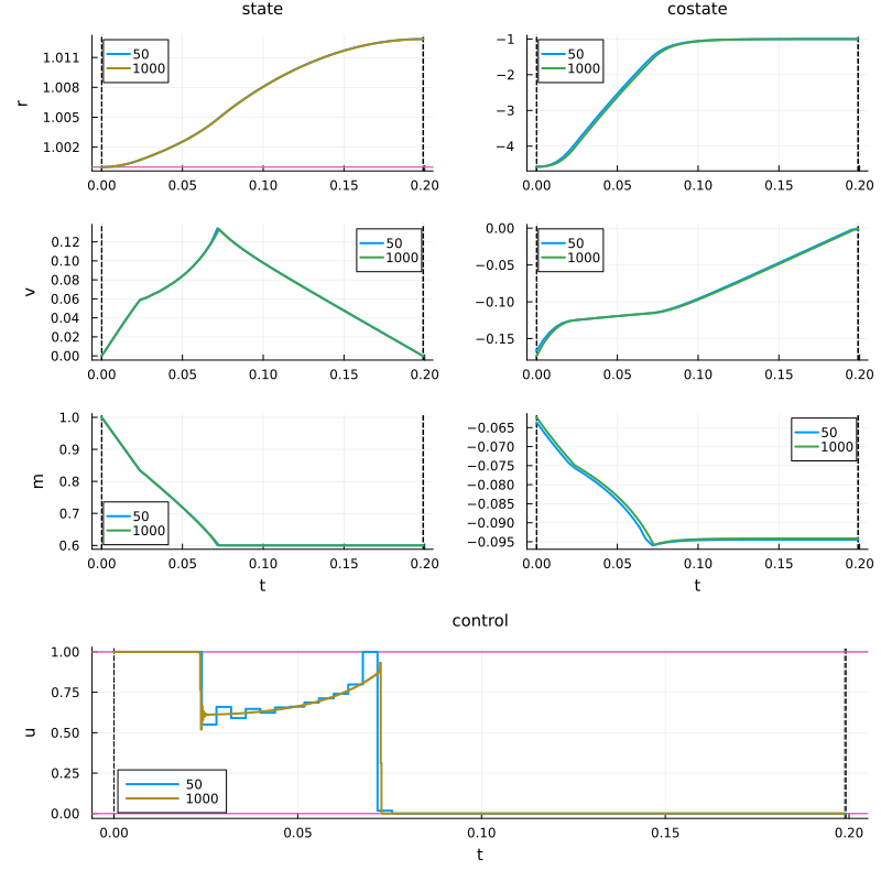
This is grid-refinement warm-starting. The very same mechanism drives parametric continuation (homotopy on a physical parameter, e.g. maximum thrust): Discrete continuation.
Comparison with a bang-bang strategy
How much better is the optimal solution compared to a naive strategy? We simulate full thrust until fuel depletion, then coast to apogee — a bang-bang profile with no optimisation, just two ODE integrations with callbacks.
using OrdinaryDiffEq   # ODE solver (callbacks for the bang-bang simulation)

# Phase 1: u = 1, stop when m = mf (fuel depleted)
bang1!(dx, x, p, t) = (dx[:] = F0(x) + F1(x))
cb_fuel = ContinuousCallback((u, t, int) -> u[3] - mf, terminate!)
sol_bang1 = solve(ODEProblem(bang1!, [r0, v0, m0], (t0, 100.0)), Tsit5(); callback=cb_fuel, reltol=1e-8, abstol=1e-8)
t1_bang, x1_bang = sol_bang1.t[end], sol_bang1[:, end]

# Phase 2: u = 0, stop when v = 0 (apogee)
bang2!(dx, x, p, t) = (dx[:] = F0(x))
cb_apogee = ContinuousCallback((u, t, int) -> u[2], terminate!)
sol_bang2 = solve(ODEProblem(bang2!, x1_bang, (t1_bang, 1000.0)), Tsit5(); callback=cb_apogee, reltol=1e-8, abstol=1e-8)
tf_bang, rf_bang = sol_bang2.t[end], sol_bang2[1, end]

println("Bang-bang: r(tf) = ", round(rf_bang, digits=6), "  (t1=", round(t1_bang, digits=4), ", tf=", round(tf_bang, digits=4), ")")
println("Optimal:   r(tf) = ", round(objective(sol_cold), digits=6), "  (           tf=", round(variable(sol_cold), digits=4), ")")
Bang-bang: r(tf) = 1.012505 (t1=0.0571, tf=0.1873)
Optimal: r(tf) = 1.012837 ( tf=0.1989)The optimal thrust profile uses a singular arc — it does not simply push at the maximum. Overlaying the two trajectories on the altitude–velocity plane makes the difference visible:
# assemble the bang-bang trajectory as (t, r, v, m) for plotting
t_bang = [sol_bang1.t; sol_bang2.t]
r_bang = [sol_bang1[1, :]; sol_bang2[1, :]]

plt_bang = plot(sol_cold; label="optimal", linewidth=2, color=1)
plot!(plt_bang[1], t_bang, r_bang; label="bang-bang", linestyle=:dash, linewidth=2, color=2)
plot(plt_bang[1]; legend=:bottomright, xlabel="time", ylabel="altitude")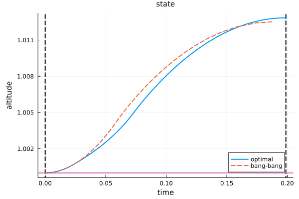
Solving on a GPU
Moving to the GPU is a single token, :gpu, which auto-completes to (:collocation, :exa, :madnlp, :gpu). It requires the :exa modeler (hence @def, not the macro-free API — cf. the definition section) plus a CUDA-capable GPU.
In a seminar or on Binder there is usually no functional GPU, so the call is expected to fail — that is the pedagogical point: the :gpu token needs a specific setup. We wrap it in a try/catch so the tour keeps running and shows the raised exception.
using MadNLPGPU
using CUDA

try
    global sol_gpu = solve(goddard, :gpu; grid_size=1000, display=false)
    println("GPU solve succeeded — a functional GPU is available.")
catch e
    println("GPU solve failed, as expected without a functional GPU.")
    println("CUDA.functional() = ", CUDA.functional())
    println("Exception: ", first(sprint(showerror, e), 400))
end
┌ Warning: CUDA is loaded but not functional. GPU backend may not work properly.
└ @ CTSolversCUDA ~/.julia/packages/CTSolvers/FGN4F/ext/CTSolversCUDA.jl:29
GPU solve failed, as expected without a functional GPU.
CUDA.functional() = false
Exception: CUDA driver not functionalFor the full GPU setup, see Solve on GPU.
The indirect method
We now return to the double integrator ocp from the earlier sections. Its shooting has just two unknowns and is initialised by the direct costate above, which makes it ideal to see the indirect method. (The Goddard shooting is a structured multi-arc problem — see the links in the last section.)
In control-toolbox we systematically pair the direct method with the indirect one, based on Pontryagin's Maximum Principle (PMP), with pseudo-Hamiltonian
\[H(x,p,u) = p\,f(x,u) + p^0 f^0(x,u) \qquad (\text{normal case } p^0 = -1).\]
The PMP gives the maximising control in feedback form
\[u(x,p) = \arg\max_u H,\]
and the optimal trajectory solves a boundary value problem that we recast as a shooting equation
\[S(p_0) = 0.\]
The indirect method proceeds in three steps:
Maximising control. The PMP yields the control in feedback form $u(x, p) = \arg\max_u H(x, p, u)$. Substituting back gives the maximised Hamiltonian
\[\mathbf{H}(x, p) = H(x, p, u(x, p)).\]
Boundary value problem. The optimal trajectory satisfies the Hamiltonian system
\[\dot{x} = \nabla_p \mathbf{H}, \qquad \dot{p} = -\nabla_x \mathbf{H},\]
with boundary conditions $x(t_0) = x_0$, $x(t_f) = x_f$.
Shooting function. Let $\varphi_{t_0, x_0, p_0}(\cdot)$ denote the flow of the Hamiltonian vector field from $(x_0, p_0)$. The shooting function
\[S(p_0) = \pi(\varphi_{t_0, x_0, p_0}(t_f)) - x_f, \qquad \pi(x, p) = x,\]
measures the miss at $t_f$: solving the BVP reduces to finding $p_0$ such that $S(p_0) = 0$.
For the energy problem, $H = p_1 v + p_2 u - u^2/2$, so the maximiser is $u = p_2$.
using OrdinaryDiffEq   # ODE solver (Hamiltonian flow)
using NonlinearSolve   # nonlinear equations (shooting)

# maximising control in feedback form
u_max(x, p) = p[2]

# Hamiltonian flow of the OCP
φ = Flow(ocp, u_max);

# state projection π(x, p) = x
proj((x, p)) = x

# shooting function
S(p0) = proj(φ(t0, x0, p0, tf)) - xf
The shooting is initialised with the costate of the direct solution — the very adjoint we highlighted above:
nle!(s, p0, _) = (s[:] = S(p0))

p_of_t   = costate(direct_sol)     # costate as a function of time
p0_guess = p_of_t(t0)              # initial costate from the direct method

prob = NonlinearProblem(nle!, p0_guess)
shooting_sol = solve(prob; show_trace=Val(true))
p0_sol = shooting_sol.u

println("costate p0 = ", p0_sol)
println("shoot S(p0) = ", S(p0_sol))
Algorithm: NewtonRaphson(
    descent = NewtonDescent(),
    autodiff = AutoForwardDiff(),
    vjp_autodiff = AutoReverseDiff(
        compile = false
    ),
    jvp_autodiff = AutoForwardDiff(),
    concrete_jac = Val{false}()
)

----    	-------------       	-----------
Iter    	f(u) inf-norm       	Step 2-norm
----    	-------------       	-----------
0       	2.40003840e-02      	0.00000000e+00
1       	1.15085180e-14      	2.39051536e-02
Final   	1.15085180e-14
----------------------
costate p0 = [12.000000000000133, 6.000000000000043]
shoot S(p0) = [3.853755692201154e-16, -1.1508517954971638e-14]
Reconstruct the indirect solution from the flow and overlay it with the direct solution:
indirect_sol = φ((t0, tf), x0, p0_sol; saveat=range(t0, tf, 100))

plt_compare = plot(direct_sol; label="direct", size=(800, 600))
plot!(plt_compare, indirect_sol; label="indirect")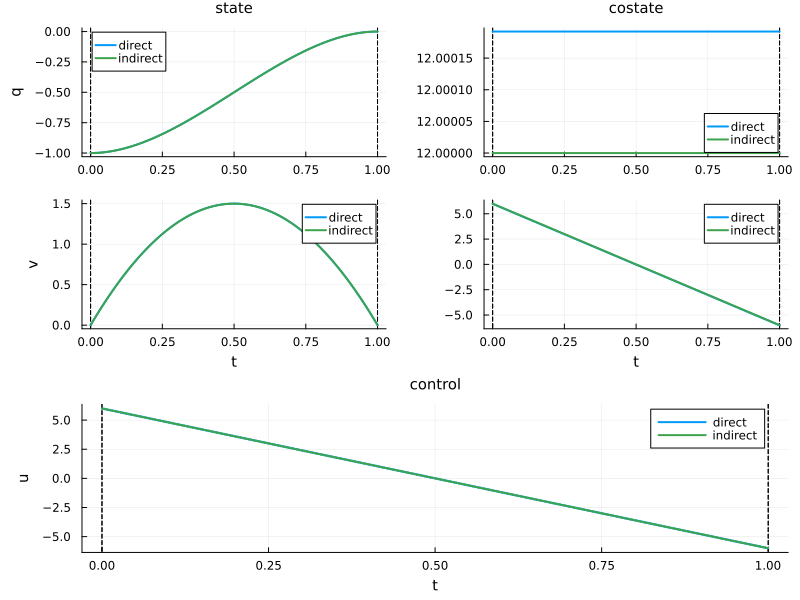
See Compute flows from optimal control problems for the flow construction, and the indirect simple shooting tutorial.
Going further
Variables & parameters. Beyond the control, one can optimise parameters naturally, both in an OCP (the variable keyword of the DSL) and in a differential-constraint optimisation problem without any control (a control-free problem). See control-free problems.
Advanced examples (each does both direct and indirect):
- Singular control (control-affine systems) — singular control
- State constraint — state constraint
- Goddard problem — free final time, a singular arc, a state constraint and a structured shooting all at once — Goddard tutorial
Discrete continuation — warm-starting across a family of problems (homotopy on a physical parameter), the grown-up version of the grid continuation above: Discrete continuation.
This page was generated using Literate.jl.