Control-free problems

Control-free problems are optimal control problems without a control variable. They are used for optimizing constant parameters in dynamical systems, such as:

• Identifying unknown parameters from observed data (parameter estimation)

• Finding optimal parameters for a given performance criterion

This page demonstrates two simple examples with known analytical solutions.

First, we import the necessary packages:

using OptimalControl
using NLPModelsIpopt
using Plots

Example 1: Exponential growth rate estimation

Consider a system with exponential growth:

where is an unknown growth rate parameter. We have observed data with some perturbations and want to estimate by minimizing the squared error:

The underlying model has  , but the observed data includes perturbations.

Problem definition

# observed data (analytical solution with λ = 0.5)
λ_true = 0.5
model(t) = 2 * exp(λ_true * t)
perturbation(t) = 2e-1*sin(4π*t)
data(t) = model(t) + perturbation(t)

# optimal control problem (parameter estimation)
t0 = 0; tf = 2; x0 = 2
ocp = @def begin
    λ ∈ R, variable              # growth rate to estimate
    t ∈ [t0, tf], time
    x ∈ R, state

    x(t0) == x0
    ẋ(t) == λ * x(t)

    ∫((x(t) - data(t))^2) → min  # fit to observed data
end

Direct method

direct_sol = solve(ocp; grid_size=20, display=false)

• Solver:
  ✓ Successful  : true
  │  Status     : first_order
  │  Message    : Ipopt/generic
  │  Iterations : 14
  │  Objective  : 0.039296407666384314
  └─ Constraints violation : 9.325873406851315e-15

• Variable: λ = 0.4960778956661449

• Boundary duals: [0.061507876561442874]

println("Estimated growth rate: λ = ", variable(direct_sol))
println("Objective value: ", objective(direct_sol))

Estimated growth rate: λ = 0.4960778956661449
Objective value: 0.039296407666384314

# plot direct solution
plt = plot(direct_sol; size=(800, 400), label="Direct")

# Add data on first plot
t_grid = time_grid(direct_sol)
plot!(plt, t_grid, data.(t_grid); subplot=1, line=:dot, lw=2, label="Data", color=:black)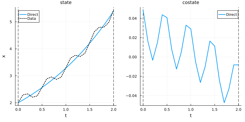

The estimated parameter should be close to  .

Indirect method

We now solve the same problem using an indirect shooting method based on Pontryagin's Maximum Principle. First, we import the necessary packages:

using OrdinaryDiffEq  # ODE solver
using NonlinearSolve  # Nonlinear solver

For control-free problems with a variable parameter, we use an augmented Hamiltonian approach. The Hamiltonian for this problem is:

To handle the variable parameter , we treat it as an additional state with zero dynamics. This gives us the augmented system with state and costate , where:

The transversality condition for the variable parameter requires   . Assuming  , we have to satisfy:

We use CTFlows' augment=true feature to automatically compute without manually constructing the augmented system.

# Create Hamiltonian flow from OCP
f = Flow(ocp)

Note

For more details about the flow construction, see this page.

The shooting function enforces the transversality conditions   and  . Using augment=true, the flow automatically returns , with   by construction.

# Shooting function: S(p0, λ) = (p(tf), pλ(tf))
# We want both components to be zero at tf
function shoot!(s, p0, λ)
    _, px_tf, pλ_tf = f(t0, x0, p0, tf, λ; augment=true)
    s[1] = px_tf
    s[2] = pλ_tf
    return nothing
end

# Auxiliary in-place NLE function
nle!(s, y, _) = shoot!(s, y...)

We use the direct solution to initialize the shooting method:

# Extract solution from direct method for initialization
p_direct = costate(direct_sol)
λ_direct = variable(direct_sol)

# Initial guess
p0_guess = p_direct(t0)
λ_guess = λ_direct

# NLE problem with initial guess (2 unknowns: p0, λ)
prob_indirect = NonlinearProblem(nle!, [p0_guess, λ_guess])

# Solve shooting equations
shooting_sol = solve(prob_indirect; show_trace=Val(false))
p0_sol, λ_sol = shooting_sol.u

println("Indirect solution:")
println("Initial costate: p0 = ", p0_sol)
println("Parameter: λ = ", λ_sol)

Indirect solution:
Initial costate: p0 = 0.058478510601397186
Parameter: λ = 0.4966212669483583

Finally, we compute and plot the indirect solution:

# Compute and plot indirect solution
indirect_sol = f((t0, tf), x0, p0_sol, λ_sol; saveat=range(t0, tf, 200))
plot!(plt, indirect_sol; linestyle=:dash, lw=2, label="Indirect", color=2)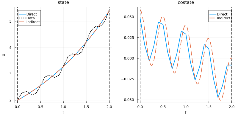

The direct and indirect solutions match closely, both fitting the perturbed observed data.

Example 2: Harmonic oscillator pulsation optimization

Consider a harmonic oscillator:

with initial conditions  ,   and final condition  . We want to find the minimal pulsation satisfying these constraints:

The analytical solution is   , giving  .

Problem definition

# optimal control problem (pulsation optimization)
q0 = 1; v0 = 0
t0 = 0; tf = 1
ocp = @def begin
    ω ∈ R, variable              # pulsation to optimize
    t ∈ [t0, tf], time
    x = (q, v) ∈ R², state

    q(t0) == q0
    v(t0) == v0
    q(tf) == 0.0                  # final condition

    ẋ(t) == [v(t), -ω^2 * q(t)]

    ω^2 → min   # minimize pulsation
end

Direct method

direct_sol = solve(ocp; grid_size=20, display=false)

• Solver:
  ✓ Successful  : true
  │  Status     : first_order
  │  Message    : Ipopt/generic
  │  Iterations : 9
  │  Objective  : 2.469940014156302
  └─ Constraints violation : 1.3778783669593508e-11

• Variable: ω = 1.5716042803951324

• Boundary duals: [2.776384949033009e-10, -2.003087424961417, 3.148060771075015]

println("Optimal pulsation: ω = ", variable(direct_sol))
println("Objective value: ω² = ", objective(direct_sol))
println("Expected: ω = π/2 ≈ 1.5708, ω² ≈ 2.4674")

Optimal pulsation: ω = 1.5716042803951324
Objective value: ω² = 2.469940014156302
Expected: ω = π/2 ≈ 1.5708, ω² ≈ 2.4674

plot(direct_sol; size=(800, 400))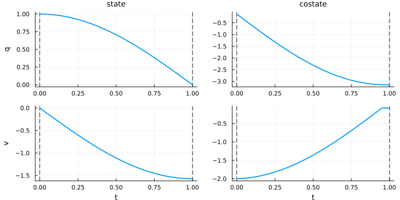

The optimal pulsation should be close to   , and the objective  .

Comparison with analytical solutions

For the harmonic oscillator, we can compare the numerical solution with the analytical one:

# analytical solution
t_analytical = range(0, 1, 100)
q_analytical = cos.(π * t_analytical / 2)
v_analytical = -(π/2) * sin.(π * t_analytical / 2)

# plot comparison
plt = plot(direct_sol; size=(800, 600), label="Direct")
plot!(plt, t_analytical, q_analytical;
      label="q (analytical)", linestyle=:dash, linewidth=2, subplot=1)
plot!(plt, t_analytical, v_analytical;
      label="v (analytical)", linestyle=:dash, linewidth=2, subplot=2)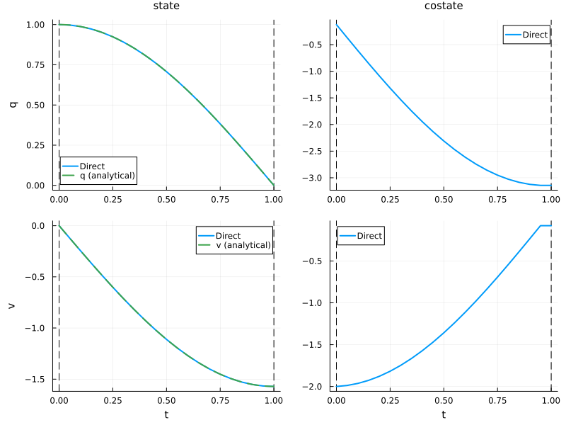

The numerical and analytical solutions should match very closely.

Indirect method

We now solve the same problem using an indirect shooting method. For this control-free problem with a variable parameter, we use an augmented Hamiltonian approach. The Hamiltonian for this problem is:

To handle the variable parameter , we treat it as an additional state with zero dynamics. This gives us the augmented system with state and costate , where:

For this problem with a Mayer cost  , the transversality condition for the variable parameter is:

Assuming  , we have:

We use CTFlows' augment=true feature to automatically compute without manually constructing the augmented system:

# Create Hamiltonian flow from OCP
f = Flow(ocp)

Note

For more details about the flow construction, see this page.

The shooting function enforces the conditions:

• Final condition:  

• Free final velocity:  

• Transversality condition for Mayer cost:   

Using augment=true, the flow automatically returns , with   by construction.

# Shooting function: S(p0, ω)
function shoot!(s, p0, ω)
    x_tf, p_tf, pω_tf = f(t0, [q0, v0], p0, tf, ω; augment=true)
    q_tf = x_tf[1]
    pv_tf = p_tf[2]
    s[1] = q_tf         # q(tf) = 0
    s[2] = pv_tf        # p2(tf) = 0 (free final velocity)
    s[3] = pω_tf + 2ω  # pω(tf) + 2ω = 0 (Mayer cost transversality)
    return nothing
end

# Auxiliary in-place NLE function
nle!(s, y, _) = shoot!(s, y[1:2], y[3])

We use the direct solution to initialize the shooting method:

# Extract solution from direct method for initialization
p_direct = costate(direct_sol)
ω_direct = variable(direct_sol)

# Initial guess
p0_guess = p_direct(t0)
ω_guess = ω_direct

# NLE problem with initial guess
prob_indirect = NonlinearProblem(nle!, [p0_guess..., ω_guess])

# Solve shooting equations
shooting_sol = solve(prob_indirect; show_trace=Val(false))
p0_sol, ω_sol = shooting_sol.u[1:2], shooting_sol.u[3]

println("Indirect solution:")
println("Initial costate: p0 = ", p0_sol)
println("Parameter: ω = ", ω_sol)

Indirect solution:
Initial costate: p0 = [7.62813477748342e-15, -2.0000000000035025]
Parameter: ω = 1.5707963267948069

Finally, we compute and plot the indirect solution:

# Compute and plot indirect solution
indirect_sol = f((t0, tf), [q0, v0], p0_sol, ω_sol; saveat=range(t0, tf, 200))
plot!(plt, indirect_sol; linestyle=:dash, lw=2, label="Indirect", color=2)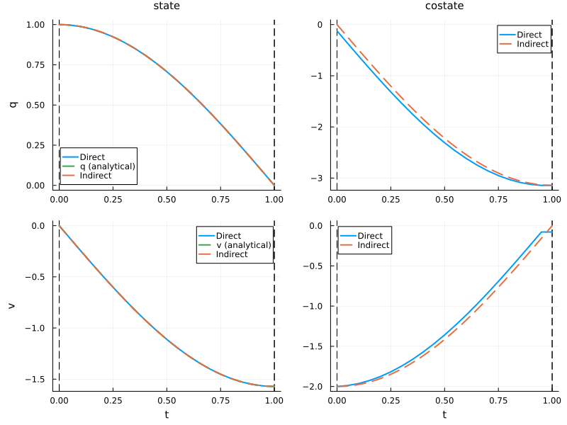

The direct and indirect solutions match closely, both finding the optimal pulsation  .

Applications

Control-free problems appear in many contexts:

• System identification: estimating physical parameters (mass, damping, stiffness) from experimental data

• Optimal design: finding optimal geometric or physical parameters (length, stiffness, etc.)

• Inverse problems: reconstructing unknown inputs or initial conditions from partial observations

See the syntax documentation for more details on defining control-free problems.