Singular control
For control-affine systems of the form
the pseudo-Hamiltonian is
When the switching function
This page demonstrates how to compute singular controls both by hand and using differential geometry tools from OptimalControl.jl, then verifies the result numerically using direct and indirect methods.
First, we import the necessary packages:
using OptimalControl
using NLPModelsIpopt
using Plots
Problem definition
We consider a vehicle moving in the plane with drift. The state is
with control constraint
We want to find the time-optimal transfer from the origin
ocp = @def begin

    tf ∈ R, variable
    t ∈ [0, tf], time
    q = (x, y, θ) ∈ R³, state
    u ∈ R, control

    -1 ≤ u(t) ≤ 1                     # Control bounds
    -π/2 ≤ θ(t) ≤ π/2                 # State bounds (helps direct method convergence)

    x(0) == 0
    y(0) == 0
    x(tf) == 1
    y(tf) == 0

    ∂(q)(t) == [cos(θ(t)), sin(θ(t)) + x(t), u(t)]

    tf → min

end
This is a control-affine system with:
Direct method
We solve the problem using a direct method:
direct_sol = solve(ocp; display=false)
println("Optimal time: tf = ", variable(direct_sol))
Optimal time: tf = 1.1497309627876084Let's plot the solution:
opt = (state_bounds_style=:none, control_bounds_style=:none)
plt = plot(direct_sol; label="Direct", size=(800, 800), opt...)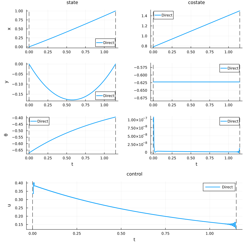
Singular control by hand
The pseudo-Hamiltonian for this time-optimal problem is:
This is control-affine:
The switching function is
First derivative:
Computing the Poisson bracket:
Since
On the singular arc,
Second derivative:
For the arc to remain singular,
whenever
Computing
Therefore:
Non-degeneracy condition
We can show that
Since this matrix has determinant 1 (hence is invertible), we would have
Simplification using the constraint:
Multiply numerator and denominator by
From the constraint
So the singular control is:
Let's overlay this on the numerical solution:
T = time_grid(direct_sol)
θ(t) = state(direct_sol)(t)[3]
us(t) = sin(θ(t))^2
plot!(plt, T, us; subplot=7, line=:dash, lw=2, label="us (hand)")
plot(plt[7]; size=(800, 400))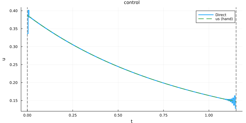
Singular control via Poisson brackets
We can compute the same result using the differential geometry tools from OptimalControl.jl. See the differential geometry tools manual for detailed explanations.
First, define the vector fields:
F0(q) = [cos(q[3]), sin(q[3]) + q[1], 0]
F1(q) = [0, 0, 1]
Compute their Hamiltonian lifts:
H0 = Lift(F0)
H1 = Lift(F1)
Compute the iterated Poisson brackets:
H01 = @Lie {H0, H1}
H001 = @Lie {H0, H01}
H101 = @Lie {H1, H01}
The singular control is:
us_bracket(q, p) = -H001(q, p) / H101(q, p)Let's verify this gives the same result:
q(t) = state(direct_sol)(t)
p(t) = costate(direct_sol)(t)
us_b(t) = us_bracket(q(t), p(t))
plot!(plt, T, us_b; subplot=7, line=:dashdot, lw=2, label="us (brackets)")
plot(plt[7]; size=(800, 400))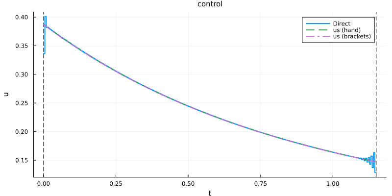
Both methods give the same singular control, which matches the numerical solution from the direct method.
Indirect shooting method
We now solve the problem using an indirect shooting method based on the singular control we computed. This approach is similar to the one used in the double integrator example.
First, import the necessary packages:
using OrdinaryDiffEq
using NonlinearSolve
Define the singular control in feedback form:
u_indirect(x) = sin(x[3])^2Build the flow for the singular arc:
f = Flow(ocp, (x, p, tf) -> u_indirect(x))Define the shooting function. We have 5 unknowns: the initial costate
t0 = 0

function shoot!(s, p0, θ0, tf)

    q_t0, p_t0 = [0, 0, θ0], p0
    q_tf, p_tf = f(t0, q_t0, p_t0, tf)

    s[1] = q_tf[1] - 1      # x(tf) = 1 (boundary condition)
    s[2] = q_tf[2]          # y(tf) = 0 (boundary condition)
    s[3] = p_t0[3]          # pθ(0) = 0 (transversality condition)
    s[4] = p_tf[3]          # pθ(tf) = 0 (transversality condition)

    # H(tf) = 1 (for time-optimal with p^0 = -1)
    pxf = p_tf[1]
    pyf = p_tf[2]
    θf = q_tf[3]
    s[5] = pxf * cos(θf) + pyf * (sin(θf) + 1) - 1

    return nothing
end
Use the direct solution to provide an initial guess:
p0 = costate(direct_sol)(t0)
θ0 = state(direct_sol)(t0)[3]
tf = variable(direct_sol)

println("Initial guess:")
println("p0 = ", p0)
println("θ0 = ", θ0)
println("tf = ", tf)
Initial guess:
p0 = [0.784064017685243, -0.6224842865890237, 9.564334353787437e-8]
θ0 = -0.6717544714481044
tf = 1.1497309627876084Set up and solve the nonlinear system:
# Auxiliary in-place NLE function
nle!(s, ξ, _) = shoot!(s, ξ[1:3], ξ[4], ξ[5])

# Initial guess for the Newton solver
ξ_guess = [p0..., θ0, tf]

# NLE problem with initial guess
prob = NonlinearProblem(nle!, ξ_guess)

# Resolution of the shooting equations
shooting_sol = solve(prob; show_trace=Val(false))
p0_sol, θ0_sol, tf_sol = shooting_sol.u[1:3], shooting_sol.u[4], shooting_sol.u[5]

println("Shooting solution:")
println("p0 = ", p0_sol)
println("θ0 = ", θ0_sol)
println("tf = ", tf_sol)
Shooting solution:
p0 = [0.7826328345972628, -0.6224836111984365, 0.0]
θ0 = -0.6719121189983684
tf = 1.1497308858208615Reconstruct the indirect solution:
indirect_sol = f((t0, tf_sol), [0, 0, θ0_sol], p0_sol; saveat=range(t0, tf_sol, 100))Plot the indirect solution alongside the direct solution:
plot!(plt, indirect_sol; label="Indirect", color=2, linestyle=:dash, opt...)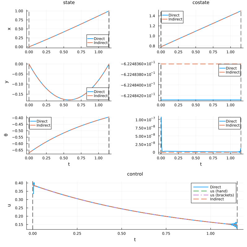
The indirect and direct solutions match very well, confirming that our singular control computation is correct.
See also
Differential geometry tools — Mathematical definitions and usage of
Lift,Poisson,@LieGoddard tutorial — More complex example with bang, singular, and boundary arcs
Compute flows from optimal control problems — Using flows for indirect methods