How to compute flows from optimal control problems

In this tutorial, we explain the Flow function, in particular to compute flows from an optimal control problem.

Basic usage

Les us define a basic optimal control problem.

using OptimalControl

t0 = 0
tf = 1
x0 = [-1, 0]

ocp = @def begin

    t ∈ [ t0, tf ], time
    x = (q, v) ∈ R², state
    u ∈ R, control

    x(t0) == x0
    x(tf) == [0, 0]
    ẋ(t)  == [v(t), u(t)]

    ∫( 0.5u(t)^2 ) → min

end

The pseudo-Hamiltonian of this problem is

where    since we are in the normal case. From the Pontryagin maximum principle, the maximising control is given in feedback form by

since     .

u(x, p) = p[2]

Actually, if is a solution of the optimal control problem, then, the Pontryagin maximum principle tells us that there exists a costate such that   and such that the pair satisfies:

The Flow function aims to compute   from the optimal control problem ocp and the control in feedback form u(x, p).

Nota bene

Actually, writing  , then the pair is also solution of

where   and   . This is what is actually computed by Flow.

Let us try to get the associated flow:

julia> f = Flow(ocp, u)
ERROR: ExtensionError. Please make: julia> using OrdinaryDiffEq

As you can see, an error occurred since we need the package OrdinaryDiffEq.jl. This package provides numerical integrators to compute solutions of the ordinary differential equation  .

OrdinaryDiffEq.jl

The package OrdinaryDiffEq.jl is part of DifferentialEquations.jl. You can either use one or the other.

using OrdinaryDiffEq
f = Flow(ocp, u)

Now we have the flow of the associated Hamiltonian vector field, we can use it. Some simple calculations shows that the initial covector solution of the Pontryagin maximum principle is . Let us check that integrating the flow from    to the final time we reach the target  .

p0 = [12, 6]
xf, pf = f(t0, x0, p0, tf)
xf

2-element Vector{Float64}:
 -1.6443649131320877e-15
  6.0194942550307896e-15

If you prefer to get the state, costate and control trajectories at any time, you can call the flow like this:

sol = f((t0, tf), x0, p0)

In this case, you obtain a data that you can plot exactly like when solving the optimal control problem with the function solve. See for instance the basic example or the plot tutorial.

using Plots
plot(sol)

You can notice from the graph of v that the integrator has made very few steps:

time_grid(sol)

6-element Vector{Float64}:
 0.0
 0.002407303553528376
 0.01626703922322027
 0.08846744312965177
 0.38065350973196377
 1.0

Time grid

The function time_grid returns the discretised time grid returned by the solver. In this case, the solution has been computed by numerical integration with an adaptive step-length Runge-Kutta scheme.

To have a better visualisation (the accuracy won't change), you can provide a fine grid.

sol = f((t0, tf), x0, p0; saveat=range(t0, tf, 100))
plot(sol)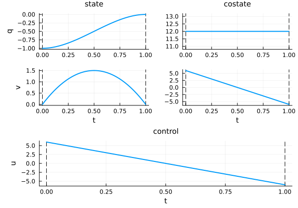

The argument saveat is an option from OrdinaryDiffEq.jl. Please check the list of common options. For instance, one can change the integrator with the keyword argument alg or the absolute tolerance with abstol. Note that you can set an option when declaring the flow or set an option in a particular call of the flow. In the following example, the integrator will be BS5() and the absolute tolerance will be abstol=1e-8.

f = Flow(ocp, u; alg=BS5(), abstol=1)   # alg=BS5(), abstol=1
xf, pf = f(t0, x0, p0, tf; abstol=1e-8) # alg=BS5(), abstol=1e-8

([-3.572529660260854e-16, -1.5425108240283176e-16], [12.0, -6.0])

Non-autonomous case

Let us consider the following optimal control problem:

t0 = 0
tf = π/4
x0 = 0
xf = tan(π/4) - 2log(√(2)/2)

ocp = @def begin

    t ∈ [t0, tf], time
    x ∈ R, state
    u ∈ R, control

    x(t0) == x0
    x(tf) == xf
    ẋ(t) == u(t) * (1 + tan(t)) # The dynamics depend explicitly on t

    0.5∫( u(t)^2 ) → min

end

The pseudo-Hamiltonian of this problem is

where    since we are in the normal case. We can notice that the pseudo-Hamiltonian is non-autonomous since it explicitly depends on the time .

is_autonomous(ocp)

false

From the Pontryagin maximum principle, the maximising control is given in feedback form by

since     .

u(t, x, p) = p * (1 + tan(t))

As before, the Flow function aims to compute from the optimal control problem ocp and the control in feedback form u(t, x, p). Since the problem is non-autonomous, we must provide a control law that depends on time.

f = Flow(ocp, u)

Now we have the flow of the associated Hamiltonian vector field, we can use it. Some simple calculations shows that the initial covector solution of the Pontryagin maximum principle is . Let us check that integrating the flow from   to the final time   we reach the target   .

p0 = 1
xf, pf = f(t0, x0, p0, tf)
xf - (tan(π/4) - 2log(√(2)/2))

-8.617551117140465e-12

Variable

Let us consider an optimal control problem with a (decision / optimisation) variable.

t0 = 0
x0 = 0

ocp = @def begin

    tf ∈ R, variable # the optimisation variable is tf
    t ∈ [t0, tf], time
    x ∈ R, state
    u ∈ R, control

    x(t0) == x0
    x(tf) == 1
    ẋ(t) == tf * u(t)

    tf + 0.5∫(u(t)^2) → min

end

As you can see, the variable is the final time tf. Note that the dynamics depends on tf. From the Pontryagin maximum principle, the solution is given by:

tf = (3/2)^(1/4)
p0 = 2tf/3

The input arguments of the maximising control are now the state x, the costate p and the variable tf.

u(x, p, tf) = tf * p

Let us check that the final condition x(tf) = 1 is satisfied.

f = Flow(ocp, u)
xf, pf = f(t0, x0, p0, tf, tf)

(1.0000000000000004, 0.7377879464668812)

The usage of the flow f is the following: f(t0, x0, p0, tf, v) where v is the variable. If one wants to compute the state at time t1 = 0.5, then, one must write:

t1 = 0.5
x1, p1 = f(t0, x0, p0, t1, tf)

(0.45180100180492255, 0.7377879464668812)

Free times

In the particular cases: the initial time t0 is the only variable, the final time tf is the only variable, or the initial and final times t0 and tf are the only variables and are in order v=(t0, tf), the times do not need to be repeated in the call of the flow:

xf, pf = f(t0, x0, p0, tf)

(1.0000000000000004, 0.7377879464668812)

Since the variable is the final time, we can make the time-reparameterisation    to normalise the time in .

ocp = @def begin

    tf ∈ R, variable
    s ∈ [0, 1], time
    x ∈ R, state
    u ∈ R, control

    x(0) == 0
    x(1) == 1
    ẋ(s) == tf^2 * u(s)

    tf + (0.5*tf)*∫(u(s)^2) → min

end

f = Flow(ocp, u)
xf, pf = f(0, x0, p0, 1, tf)

(1.0000000000000002, 0.7377879464668812)

Another possibility is to add a new state variable . The problem has no variable anymore.

ocp = @def begin

    s ∈ [0, 1], time
    y = (x, tf) ∈ R², state
    u ∈ R, control

    x(0) == 0
    x(1) == 1
    dx = tf(s)^2 * u(s)
    dtf = 0 * u(s) # 0
    ẏ(s) == [dx, dtf]

    tf(1) + 0.5∫(tf(s) * u(s)^2) → min

end

u(y, q) = y[2] * q[1]

f = Flow(ocp, u)
yf, pf = f(0, [x0, tf], [p0, 0], 1)

([1.0000000000000002, 1.1066819197003217], [0.7377879464668812, -1.0000000000000004])

Bug

Note that in the previous optimal control problem, we have dtf = 0 * u(s) instead of dtf = 0. The latter does not work.

Goddard problem

In the Goddard problem, you may find other constructions of flows, especially for singular and boundary arcs.

Augmented costate computation with augment=true

When working with optimal control problems that have variables, it can be useful to compute the costate associated with the variable parameter. The augment=true keyword argument provides automatic computation of this costate without requiring manual construction of the augmented Hamiltonian system.

Mathematical background

For an optimal control problem with Hamiltonian , where is the state, is the costate, and is a variable parameter, the augmented system treats the variable as an additional state with zero dynamics:

With the initial condition  , the final costate represents the accumulated sensitivity:

Usage

Let us consider a harmonic oscillator problem where the pulsation is a variable parameter appearing in the dynamics:

q0 = 1
v0 = 0
t0 = 0
tf = 1

ocp_aug = @def begin
    ω ∈ R, variable              # pulsation to optimize
    t ∈ [t0, tf], time
    x = (q, v) ∈ R², state
    u ∈ R, control

    q(t0) == q0
    v(t0) == v0
    q(tf) == 0.0

    ẋ(t) == [v(t), -ω^2 * q(t) + u(t)]

    ω^2 + 0.5∫(u(t)^2) → min
end

# Maximizing control from Pontryagin's principle
u_aug(x, p, ω) = p[2]
f_aug = Flow(ocp_aug, u_aug)

Without augment=true, the flow returns only the state and costate:

ω_val = π/2
p0_val = [1.0, 0.5]
xf, pf = f_aug(t0, [q0, v0], p0_val, tf, ω_val)
println("q(tf) = ", xf[1], ", v(tf) = ", xf[2])

q(tf) = 0.030148805356911515, v(tf) = -1.7299512698856503

With augment=true, the flow automatically computes and returns the costate associated with the variable ω:

xf, pf, pω = f_aug(t0, [q0, v0], p0_val, tf, ω_val; augment=true)
println("q(tf) = ", xf[1], ", v(tf) = ", xf[2], ", p_ω(tf) = ", pω)

q(tf) = 0.030148805358156082, v(tf) = -1.7299512698862414, p_ω(tf) = 0.12406405793461993

The value pω represents the sensitivity of the Hamiltonian with respect to the pulsation parameter:

with   by construction. This is particularly useful for computing transversality conditions in control-free problems.

Advantages

The augment=true feature provides several benefits:

• No manual work: No need to manually construct the augmented Hamiltonian or augmented ODEs

• Type-safe: Automatic handling of scalar vs vector variables

• Robust: Uses the existing, well-tested Flow(Hamiltonian(...)) infrastructure

• Mathematical rigor: Proper initial conditions and transversality handling

Error handling

The augment=true option is only available for problems with variables:

# This will throw an error (no variable in the problem)
ocp_no_var = @def begin
    t ∈ [0, 1], time
    x ∈ R, state
    u ∈ R, control
    x(0) == 0
    ẋ(t) == u(t)
    ∫(u(t)^2) → min
end

f_no_var = Flow(ocp_no_var, (x, p) -> p)
f_no_var(0, 0, 1, 1; augment=true)  # ERROR: PreconditionError

Additionally, augment=true only works for point evaluation, not for trajectory computation:

# This works (point evaluation)
xf, pf, pvf = f_aug(t0, x0, p0, tf, v; augment=true)

# This will throw an error (trajectory call)
sol = f_aug((t0, tf), x0, p0, v; augment=true)  # ERROR: PreconditionError

Control-free problems

The augment=true feature is particularly useful for control-free problems where the variable parameter appears in the dynamics. See the control-free problems example for detailed applications with transversality conditions.

Concatenation of arcs

In this part, we present how to concatenate several flows. Let us consider the following problem.

t0 =  0
tf =  1
x0 = -1
xf =  0

@def ocp begin

    t ∈ [ t0, tf ], time
    x ∈ R, state
    u ∈ R, control

    x(t0) == x0
    x(tf) == xf
    -1 ≤ u(t) ≤ 1
    ẋ(t) == -x(t) + u(t)

    ∫( abs(u(t)) ) → min

end

From the Pontryagin maximum principle, the optimal control is a concatenation of an off arc ( ) followed by a positive bang arc ( ). The initial costate is

and the switching time is   .

p0 = 1/( x0 - (xf-1) * exp(tf) )
t1 = -log(p0)

Let us define the two flows and the concatenation. Note that the concatenation of two flows is a flow.

f0 = Flow(ocp, (x, p) -> 0)     # off arc: u = 0
f1 = Flow(ocp, (x, p) -> 1)     # positive bang arc: u = 1

f = f0 * (t1, f1)               # f0 followed by f1 whenever t ≥ t1

Now, we can check that the state reach the target.

sol = f((t0, tf), x0, p0)
plot(sol)

Goddard problem

In the Goddard problem, you may find more complex concatenations.

For the moment, this concatenation is not equivalent to an exact concatenation.

f = Flow(x ->  x)
g = Flow(x -> -x)

x0 = 1
φ(t) = (f * (t/2, g))(0, x0, t)
ψ(t) = g(t/2, f(0, x0, t/2), t)

println("φ(t) = ", abs(φ(1)-x0))
println("ψ(t) = ", abs(ψ(1)-x0))

t = range(1, 5e2, 201)

plt = plot(yaxis=:log, legend=:bottomright, title="Comparison of concatenations", xlabel="t")
plot!(plt, t, t->abs(φ(t)-x0), label="OptimalControl")
plot!(plt, t, t->abs(ψ(t)-x0), label="Classical")

State constraints

We consider an optimal control problem with a state constraints of order 1.^[1]

t0 = 0
tf = 2
x0 = 1
xf = 1/2
lb = 0.1

ocp = @def begin

    t ∈ [t0, tf], time
    x ∈ R, state
    u ∈ R, control

    -1 ≤ u(t) ≤ 1
    x(t0) == x0
    x(tf) == xf
    x(t) - lb ≥ 0 # state constraint
    ẋ(t) == u(t)

    ∫( x(t)^2 ) → min

end

The pseudo-Hamiltonian of this problem is

where $ p^0 = -1 $ since we are in the normal case, and where   . Along a boundary arc, when  , we have  , so $ x(\cdot) $ is constant. Differentiating, we obtain   . Hence, along a boundary arc, the control in feedback form is:

From the maximisation condition, along a boundary arc, we have  . Differentiating, we obtain    . Hence, along a boundary arc, the dual variable is given in feedback form by:

Note

Within OptimalControl.jl, the constraint must be given in the form:

c([t, ]x, u[, v])

the control law in feedback form must be given as:

u([t, ]x, p[, v])

and the dual variable:

μ([t, ]x, p[, v])

The time t must be provided when the problem is non-autonomous and the variable v must be given when the optimal control problem contains a variable to optimise.

The optimal control is a concatenation of 3 arcs: a negative bang arc followed by a boundary arc, followed by a positive bang arc. The initial covector is approximately   , the first switching time is  , and the exit time of the boundary is  . Let us check this by concatenating the three flows.

u(x) = 0     # boundary control
c(x) = x-lb  # constraint
μ(x) = 2x    # dual variable

f1 = Flow(ocp, (x, p) -> -1)
f2 = Flow(ocp, (x, p) -> u(x), (x, u) -> c(x), (x, p) -> μ(x))
f3 = Flow(ocp, (x, p) -> +1)

t1 = 0.9
t2 = 1.6
f = f1 * (t1, f2) * (t2, f3)

p0 = -0.982237546583301
xf, pf = f(t0, x0, p0, tf)
xf

0.5000000005530089

Jump on the costate

Let consider the following problem:

t0=0
tf=1
x0=[0, 1]
l = 1/9
@def ocp begin
    t ∈ [ t0, tf ], time
    x ∈ R², state
    u ∈ R, control
    x(t0) == x0
    x(tf) == [0, -1]
    x₁(t) ≤ l,                      (x_con)
    ẋ(t) == [x₂(t), u(t)]
    0.5∫(u(t)^2) → min
end

The pseudo-Hamiltonian of this problem is

where $ p^0 = -1 $ since we are in the normal case, and where the constraint is    . Along a boundary arc, when  , we have  , so   . Differentiating again, we obtain    (the constraint is of order 2). Hence, along a boundary arc, the control in feedback form is:

From the maximisation condition, along a boundary arc, we have  . Differentiating, we obtain    . Differentiating again, we obtain   . Hence, along a boundary arc, the Lagrange multiplier is given in feedback form by:

Outside a boundary arc, the maximisation condition gives  . A deeper analysis of the problem shows that the optimal solution has 3 arcs, the first and the third ones are interior to the constraint. The second arc is a boundary arc, that is   along the second arc. We denote by and the two switching times. We have    and    , since  . The initial costate solution is    .

Important

The costate is discontinuous at and with a jump of .

Let us compute the solution concatenating the flows with the jumps.

t1 = 3l
t2 = 1 - 3l
p0 = [-18, -6]

fs = Flow(ocp,
    (x, p) -> p[2]      # control along regular arc
    )
fc = Flow(ocp,
    (x, p) -> 0,        # control along boundary arc
    (x, u) -> l-x[1],   # state constraint
    (x, p) -> 0         # Lagrange multiplier
    )

ν = 18  # jump value of p1 at t1 and t2

f = fs * (t1, [ν, 0], fc) * (t2, [ν, 0], fs)

xf, pf = f(t0, x0, p0, tf) # xf should be [0, -1]

([9.932368061361347e-17, -0.9999999999999993], [18.0, -5.999999999999999])

Let us solve the problem with a direct method to compare with the solution from the flow.

using NLPModelsIpopt

direct_sol = solve(ocp)
plot(direct_sol; label="direct", size=(800, 700))

flow_sol = f((t0, tf), x0, p0; saveat=range(t0, tf, 100))
plot!(flow_sol; label="flow", state_style=(color=3,), linestyle=:dash)

---

1. B. Bonnard, L. Faubourg, G. Launay & E. Trélat, Optimal Control With State Constraints And The Space Shuttle Re-entry Problem, J. Dyn. Control Syst., 9 (2003), no. 2, 155–199. ↩︎