How to compute Hamiltonian flows and trajectories

In this tutorial, we explain the Flow function, in particular to compute flows from a Hamiltonian vector fields, but also from general vector fields.

Introduction

Consider the simple optimal control problem from the basic example page. The pseudo-Hamiltonian is

where  ,  ,    since we are in the normal case. From the Pontryagin maximum principle, the maximising control is given in feedback form by

since     .

u(x, p) = p[2]

Actually, if is a solution of the optimal control problem, then, the Pontryagin maximum principle tells us that there exists a costate such that   and such that the pair satisfies:

Nota bene

Actually, writing  , then the pair is also solution of

where   and   .

Let us import the necessary packages.

using OptimalControl
using OrdinaryDiffEq

The package OrdinaryDiffEq.jl provides numerical integrators to compute solutions of ordinary differential equations.

OrdinaryDiffEq.jl

The package OrdinaryDiffEq.jl is part of DifferentialEquations.jl. You can either use one or the other.

Extremals from the Hamiltonian

The pairs solution of the Hamitonian vector field are called extremals. We can compute some constructing the flow from the optimal control problem and the control in feedback form. Another way to compute extremals is to define explicitly the Hamiltonian.

H(x, p, u) = p[1] * x[2] + p[2] * u - 0.5 * u^2     # pseudo-Hamiltonian
H(x, p) = H(x, p, u(x, p))                          # Hamiltonian

z = Flow(OptimalControl.Hamiltonian(H))

t0 = 0
tf = 1
x0 = [-1, 0]
p0 = [12, 6]
xf, pf = z(t0, x0, p0, tf)

([-1.6443649131320877e-15, 6.0194942550307896e-15], [12.0, -5.999999999999998])

Extremals from the Hamiltonian vector field

You can also provide the Hamiltonian vector field.

Hv(x, p) = [x[2], p[2]], [0.0, -p[1]]     # Hamiltonian vector field

z = Flow(OptimalControl.HamiltonianVectorField(Hv))
xf, pf = z(t0, x0, p0, tf)

([-1.6443649131320877e-15, 6.0194942550307896e-15], [12.0, -5.999999999999998])

Note that if you call the flow on tspan=(t0, tf), then you obtain the output solution from OrdinaryDiffEq.jl.

sol = z((t0, tf), x0, p0)
xf, pf = sol(tf)[1:2], sol(tf)[3:4]

([-1.5068423663888169e-15, 2.362238023816946e-14], [12.0, -5.999999999999964])

Trajectories

You can also compute trajectories from the control dynamics   and a control law  .

u(t) = 6-12t
x = Flow((t, x) -> [x[2], u(t)]; autonomous=false) # the vector field depends on t
x(t0, x0, tf)

2-element Vector{Float64}:
 -8.881784197001252e-16
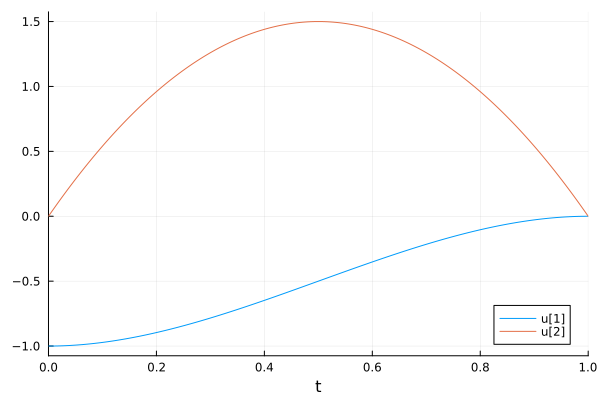
 -4.440892098500626e-16

Again, giving a tspan you get an output solution from OrdinaryDiffEq.jl.

using Plots
sol = x((t0, tf), x0)
plot(sol)