Navigation problem, MPC approach
We consider a ship in a constant current $w=(w_x,w_y)$, where $\|w\|<1$. The heading angle is controlled, leading to the following differential equations:
\[\begin{array}{rcl} \dot{x}(t) &=& w_x + \cos\theta(t), \quad t \in [0, t_f] \\ \dot{y}(t) &=& w_y + \sin\theta(t), \\ \dot{\theta}(t) &=& u(t). \end{array}\]
The state and control variables represent:
- the ship's position in the plane $(x, y)$
- the heading angle $\theta$ (direction of the ship's velocity relative to the x-axis)
- the angular velocity $u$ (rate of change of the heading angle)
The angular velocity is limited and normalized: $\|u(t)\| \leq 1$. There are boundary conditions at the initial time $t=0$ and at the final time $t=t_f$, on the position $(x,y)$ and on the angle $\theta$. The objective is to minimize the final time.
The condition $\|w\|<1$ ensures that the ship can always make progress against the current, since the ship's own velocity has unit magnitude.
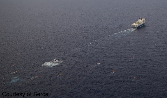
This topic stems from a collaboration between the University Côte d'Azur and the French company CGG, which is interested in optimal maneuvers of very large ships for marine exploration.
Data
using LinearAlgebra
using NLPModelsIpopt
using OptimalControl
using OrdinaryDiffEq
using Plots
using Plots.PlotMeasures
using Printf

t0 = 0.
x0 = 0.
y0 = 0.
θ0 = π/7
xf = 4.
yf = 7.
θf = -π/2

# Current model: combines a constant base current with a position-dependent perturbation.
# The parameter ε controls the magnitude of the spatial variation, while the base
# current w = [0.6, 0.4] represents the mean flow direction.
function current(x, y) # current as a function of position
    ε = 1e-1
    w = [ 0.6, 0.4 ]
    δw = ε * [ y, -x ] / sqrt(1+x^2+y^2)
    w = w + δw
    if (w[1]^2 + w[2]^2 >= 1)
        error("|w| >= 1")
    end
    return w
endClick to unfold the plotting functions.
function plot_state!(plt, x, y, θ; color=1)
    plot!(plt, [x], [y], marker=:circle, legend=false, color=color, markerstrokecolor=color, markersize=5, z_order=:front)
    quiver!(plt, [x], [y], quiver=([cos(θ)], [sin(θ)]), color=color, linewidth=2, z_order=:front)
    return plt
end

function plot_current!(plt; current=current, N=10, scaling=1)
    for x ∈ range(xlims(plt)..., N)
        for y ∈ range(ylims(plt)..., N)
            w = scaling*current(x, y)
            quiver!(plt, [x], [y], quiver=([w[1]], [w[2]]), color=:black, linewidth=0.5, z_order=:back)
        end
    end
    return plt
end

function plot_trajectory!(plt, t, x, y, θ; N=5) # N: number of points where we will display θ

    # trajectory
    plot!(plt, x.(t), y.(t), legend=false, color=1, linewidth=2, z_order=:front)

    if N > 0

        # length of the path
        s = 0
        for i ∈ 2:length(t)
            s += norm([x(t[i]), y(t[i])] - [x(t[i-1]), y(t[i-1])])
        end

        # interval of length
        Δs = s/(N+1)
        tis = []
        s = 0
        for i ∈ 2:length(t)
            s += norm([x(t[i]), y(t[i])] - [x(t[i-1]), y(t[i-1])])
            if s > Δs && length(tis) < N
                push!(tis, t[i])
                s = 0
            end
        end

        # display intermediate points
        for ti ∈ tis
            plot_state!(plt, x(ti), y(ti), θ(ti); color=1)
        end

    end

    return plt

end
# Display the boundary conditions and the current in the augmented phase plane
plt = plot(
xlims=(-2, 6),
ylims=(-1, 8),
size=(600, 600),
aspect_ratio=1,
xlabel="x",
ylabel="y",
title="Boundary Conditions",
leftmargin=5mm,
bottommargin=5mm,
)
plot_state!(plt, x0, y0, θ0; color=2)
plot_state!(plt, xf, yf, θf; color=2)
annotate!([(x0, y0, ("q₀", 12, :top)), (xf, yf, ("qf", 12, :bottom))])
plot_current!(plt)
OptimalControl solver
function solve(t0, x0, y0, θ0, xf, yf, θf, w;
    grid_size=300, tol=1e-8, max_iter=500, print_level=4, display=true, scheme=:euler)

    # Definition of the problem
    ocp = @def begin

        tf ∈ R, variable
        t ∈ [t0, tf], time
        q = (x, y, θ) ∈ R³, state
        u ∈ R, control

        -1 ≤ u(t) ≤ 1
        -2 ≤ x(t) ≤ 4.25
        -2 ≤ y(t) ≤ 8
        -2π ≤ θ(t) ≤ 2π

        q(t0) == [x0, y0, θ0]
        q(tf) == [xf, yf, θf]

        q̇(t) == [ w[1]+cos(θ(t)),
                  w[2]+sin(θ(t)),
                  u(t)]

        tf → min

    end

    # Initialization
    tf_init = 1.5*norm([xf, yf]-[x0, y0])
    init = @init ocp begin
        tf := tf_init
        q(t) := [ x0, y0, θ0 ] * (tf_init-t)/(tf_init-t0) + [xf, yf, θf] * (t-t0)/(tf_init-t0)
        u(t) := (θf - θ0) / (tf_init-t0)
    end

    # Resolution
    sol = OptimalControl.solve(ocp;
        init=init,
        grid_size=grid_size,
        tol=tol,
        max_iter=max_iter,
        print_level=print_level,
        display=display,
        scheme=scheme,
    )

    # Retrieval of useful data
    t = time_grid(sol)
    q = state(sol)
    x = t -> q(t)[1]
    y = t -> q(t)[2]
    θ = t -> q(t)[3]
    u = control(sol)
    tf = variable(sol)

    return t, x, y, θ, u, tf, iterations(sol), sol.solver_infos.constraints_violation

end
First resolution
We consider a constant current, and we solve a first time the problem. The current is evaluated at the initial position and assumed to remain constant throughout the trajectory.
# Resolution
t, x, y, θ, u, tf, iter, cons = solve(t0, x0, y0, θ0, xf, yf, θf, current(x0, y0); display=false);

println("Iterations: ", iter)
println("Constraints violation: ", cons)
println("tf: ", tf)
Iterations: 61
Constraints violation: 4.737095160578519e-10
tf: 9.969251026117748The solution provides:
- The optimal final time
tf: the minimum time needed to reach the target - The optimal state trajectory $(x(t), y(t), \theta(t))$
- The optimal control $u(t)$: the angular velocity profile
# Displaying the trajectory
plt_q = plot(xlims=(-2, 6), ylims=(-1, 8), aspect_ratio=1, xlabel="x", ylabel="y")
plot_state!(plt_q, x0, y0, θ0; color=2)
plot_state!(plt_q, xf, yf, θf; color=2)
plot_current!(plt_q; current=(x, y) -> current(x0, y0))
plot_trajectory!(plt_q, t, x, y, θ)

# Displaying the control
plt_u = plot(t, u; color=1, legend=false, linewidth=2, xlabel="t", ylabel="u")

# Final display
plot(plt_q, plt_u;
    layout=(1, 2),
    size=(1200, 600),
    leftmargin=5mm,
    bottommargin=5mm,
    plot_title="Constant Current Simulation"
)
The trajectory shows the ship's path when assuming the current is constant and equal to its value at the initial position.
Simulation of the Real System
In the previous simulation, we assumed that the current is constant. However, from a practical standpoint, the current depends on the position $(x, y)$. Given a current model, provided by the function current, we can simulate the actual trajectory of the ship, as long as we have the initial condition and the control over time.
Click to unfold the simulation code.
function realistic_trajectory(tf, t0, x0, y0, θ0, u, current; abstol=1e-12, reltol=1e-12, saveat=[])

    function rhs!(dq, q, dummy, t)
        x, y, θ = q
        w = current(x, y)
        dq[1] = w[1] + cos(θ)
        dq[2] = w[2] + sin(θ)
        dq[3] = u(t)
    end

    q0 = [x0, y0, θ0]
    tspan = (t0, tf)
    ode = ODEProblem(rhs!, q0, tspan)
    sol = OrdinaryDiffEq.solve(ode, Tsit5(), abstol=abstol, reltol=reltol, saveat=saveat)

    t = sol.t
    x = t -> sol(t)[1]
    y = t -> sol(t)[2]
    θ = t -> sol(t)[3]

    return t, x, y, θ

end
# Realistic trajectory
t, x, y, θ = realistic_trajectory(tf, t0, x0, y0, θ0, u, current)
# Displaying the trajectory
plt_q = plot(xlims=(-2, 6), ylims=(-1, 8), aspect_ratio=1, xlabel="x", ylabel="y")
plot_state!(plt_q, x0, y0, θ0; color=2)
plot_state!(plt_q, xf, yf, θf; color=2)
plot_current!(plt_q; current=current)
plot_trajectory!(plt_q, t, x, y, θ)
plot_state!(plt_q, x(tf), y(tf), θ(tf); color=3)
# Displaying the control
plt_u = plot(t, u; color=1, legend=false, linewidth=2, xlabel="t", ylabel="u")
# Final display
plot(plt_q, plt_u;
layout=(1, 2),
size=(1200, 600),
leftmargin=5mm,
bottommargin=5mm,
plot_title="Simulation with Current Model"
)
Note that the final position (shown in red) differs from the target position (shown in orange). This discrepancy occurs because the control was computed assuming a constant current, but the actual current varies with position. The ship drifts due to the unmodeled spatial variation of the current.
MPC Approach
In practice, we do not have the actual current data for the entire trajectory in advance, which is why we will regularly recalculate the optimal control. The idea is to update the optimal control at regular time intervals, taking into account the current at the position where the ship is located. We are therefore led to solve a number of problems with constant current, with this being updated regularly. This is an introduction to the so-called Model Predictive Control (MPC) methods.
The MPC algorithm works as follows:
- At each iteration, measure the current at the ship's current position
- Solve an optimal control problem assuming this current is constant over the entire remaining trajectory
- Apply the optimal control for a fixed time step
Δt - Simulate the ship's motion using the actual position-dependent current
- Update the ship's position and repeat until reaching the target
The parameters are:
Nmax: maximum number of MPC iterations (safety limit)ε: convergence tolerance - the algorithm stops when within this distance of the targetΔt: prediction horizon - how long to apply each computed control before re-planningP: number of discretization points for the optimal control solver
function MPC(t0, x0, y0, θ0, xf, yf, θf, current)

    Nmax = 20   # maximum number of iterations for the MPC method
    ε = 1e-1    # radius on the final condition to stop calculations
    Δt = 1.0    # fixed time step for the MPC method
    P = 300      # number of discretization points for the solver

    t1 = t0
    x1 = x0
    y1 = y0
    θ1 = θ0

    data = []

    N = 1
    stop = false

    while !stop

        # Retrieve the current at the current position
        w = current(x1, y1)

        # Solve the problem
        t, x, y, θ, u, tf, iter, cons = solve(t1, x1, y1, θ1, xf, yf, θf, w; grid_size=P, display=false);

        # Calculate the next time
        if (t1 + Δt < tf)
            t2 = t1 + Δt
        else
            t2 = tf
            stop = true
        end

        # Store the data: the current initial time, the next time, the control
        push!(data, (t2, t1, x(t1), y(t1), θ(t1), u, tf))

        # Update the parameters of the MPC method: simulate reality
        t, x, y, θ = realistic_trajectory(t2, t1, x1, y1, θ1, u, current)
        t1 = t2
        x1 = x(t1)
        y1 = y(t1)
        θ1 = θ(t1)

        # Calculate the distance to the target position
        distance = norm([x1, y1, θ1] - [xf, yf, θf])
        if N == 1
            println("     N    Distance  Iterations   Constraints       tf")
            println("------------------------------------------------------")
        end
        @printf("%6d", N)
        @printf("%12.4f", distance)
        @printf("%12d", iter)
        @printf("%14.4e", cons)
        @printf("%10.4f\n", tf)
        if !((distance > ε) && (N < Nmax))
            stop = true
        end

        #
        N += 1

    end

    return data
end

data = MPC(t0, x0, y0, θ0, xf, yf, θf, current)
N Distance Iterations Constraints tf
------------------------------------------------------
1 7.1694 61 4.7371e-10 9.9693
2 6.6190 32 1.5715e-09 11.5842
3 6.8264 22 4.5864e-10 12.1924
4 6.8259 63 1.0015e-10 12.4912
5 6.8559 32 7.2378e-11 12.6676
6 6.9181 31 3.9740e-13 12.7971
7 7.0123 33 1.7364e-10 12.8918
8 7.1406 40 1.7165e-10 12.9639
9 6.6643 38 4.7184e-15 13.3356
10 5.5541 41 1.3572e-02 13.3473
11 3.9308 95 1.0643e-02 13.3271
12 2.0681 30 3.5124e-10 13.2814
13 0.3839 215 4.4472e-05 13.2712
14 0.0324 80 1.0695e-04 13.2785Display
The final plot shows:
- The complete MPC trajectory (blue) composed of segments from each iteration
- Starting points of each segment (orange) where re-planning occurs
- The final position reached (red) - note that it is much closer to the target than in the constant-current simulation
- The control profile (right) showing the piecewise re-planning strategy
The MPC approach successfully compensates for the spatial variation of the current by continuously updating the control based on local current measurements.
# Trajectory
plt_q = plot(xlims=(-2, 6), ylims=(-1, 8), aspect_ratio=1, xlabel="x", ylabel="y")

# Final condition
plot_state!(plt_q, xf, yf, θf; color=2)

# Current
plot_current!(plt_q; current=current)

# Control
plt_u = plot(xlabel="t", ylabel="u")

for d ∈ data

    t2, t1, x1, y1, θ1, u, tf = d

    # Calculate the actual trajectory
    t, x, y, θ = realistic_trajectory(t2, t1, x1, y1, θ1, u, current)

    # Trajectory
    plot_state!(plt_q, x1, y1, θ1; color=2)
    plot_trajectory!(plt_q, t, x, y, θ; N=0)

    # Control
    plot!(plt_u, t, u; color=1, legend=false, linewidth=2)

end

# last point
d = data[end]
t2, t1, x1, y1, θ1, u, tf = d
t, x, y, θ = realistic_trajectory(t2, t1, x1, y1, θ1, u, current)
plot_state!(plt_q, x(tf), y(tf), θ(tf); color=3)

#
plot(plt_q, plt_u;
    layout=(1, 2),
    size=(1200, 600),
    leftmargin=5mm,
    bottommargin=5mm,
    plot_title="Simulation with Current Model"
)