Plot a solution
A solution of an OptimalControl modeling is an OptimalControl solution: plot draws its state, costate and control. A solved JuMP model becomes one with solution, so the two are drawn the same way, one over the other.
julia
using OptimalControl, JuMP, Ipopt, NLPModelsIpopt, OptimalControlProblems
using Plots

pb = beam(OptimalControlBackend())
N = grid_size_data(:beam, OptimalControlBackend())
sol = solve(
    model(pb), :collocation, :adnlp, :ipopt;
    init=initial_guess(pb), grid_size=N, scheme=:trapeze, display=false,
)
plot(sol)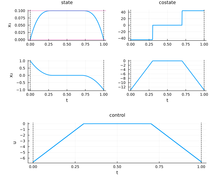
A JuMP solution over an OptimalControl one
julia
nlp = beam(JuMPBackend(); grid_size=N)
set_optimizer(nlp, Ipopt.Optimizer)
set_silent(nlp)
optimize!(nlp)

plt = plot(sol; label="OptimalControl")
plot!(plt, solution(nlp, pb); label="JuMP", linestyle=:dash)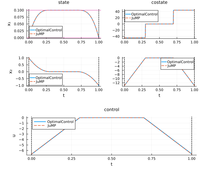
The costates of the JuMP models have the sign convention of the OptimalControl ones (-JuMP.dual, #326): the two solutions are drawn over each other.
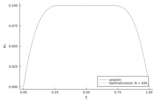
The analytic solution
When the continuous problem has a known solution, it is in the metadata, as functions of the time:
julia
exact = OptimalControlProblems.reference_solution_data(:beam)
t = range(0, 1; length=200)
plot(t, t -> exact.state(t)[1]; label="analytic", xlabel="t", ylabel="x₁")
plot!(time_grid(sol), t -> state(sol)(t)[1]; label="OptimalControl, N = $(N)", linestyle=:dash)