Double integrator: energy minimisation

Let us consider a wagon moving along a rail, whom acceleration can be controlled by a force $u$. We denote by $x = (x_1, x_2)$ the state of the wagon, that is its position $x_1$ and its velocity $x_2$.

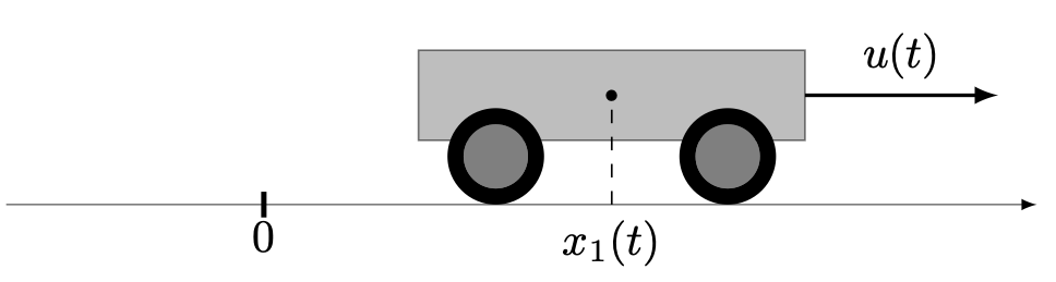
We assume that the mass is constant and unitary and that there is no friction. The dynamics we consider is given by

\[ \dot x_1(t) = x_2(t), \quad \dot x_2(t) = u(t),\quad u(t) \in \R,\]

which is simply the double integrator system. Les us consider a transfer starting at time $t_0 = 0$ and ending at time $t_f = 1$, for which we want to minimise the transfer energy

\[ \frac{1}{2}\int_{0}^{1} u^2(t) \, \mathrm{d}t\]

starting from the condition $x(0) = (-1, 0)$ and with the goal to reach the target $x(1) = (0, 0)$.

First, we need to import the OptimalControl.jl package to define the optimal control problem and NLPModelsIpopt.jl to solve it. We also need to import the Plots.jl package to plot the solution.

using OptimalControl
using NLPModelsIpopt
using Plots

<< @example-block not executed in draft mode >>

Optimal control problem

Let us define the problem with the @def macro:

ocp = @def begin
    t ∈ [0, 1], time
    x ∈ R², state
    u ∈ R, control
    x(0) == [-1, 0]
    x(1) == [0, 0]
    ẋ(t) == [x₂(t), u(t)]
    ∫( 0.5u(t)^2 ) → min
end
nothing # hide

<< @example-block not executed in draft mode >>

Nota bene

For a comprehensive introduction to the syntax used above to define the optimal control problem, check this abstract syntax tutorial. In particular, there are non-unicode alternatives for derivatives, integrals, etc.

Solve and plot

We can solve it simply with:

sol = solve(ocp)
nothing # hide

<< @example-block not executed in draft mode >>

And plot the solution with:

plot(sol)

<< @example-block not executed in draft mode >>

Nota bene

The solve function has options, see the solve tutorial. You can customise the plot, see the plot tutorial.

State constraint

We add the path constraint

\[x_2(t) \le 1.2.\]

Let us model, solve and plot the optimal control problem with this constraint.

ocp = @def begin

    t ∈ [0, 1], time
    x ∈ R², state
    u ∈ R, control

    x₂(t) ≤ 1.2

    x(0) == [-1, 0]
    x(1) == [0, 0]

    ẋ(t) == [x₂(t), u(t)]

    ∫( 0.5u(t)^2 ) → min

end

sol = solve(ocp)

plot(sol)

<< @example-block not executed in draft mode >>

Exporting and importing the solution

We can export (or save) the solution in a Julia .jld2 data file and reload it later, and also export a discretised version of the solution in a more portable JSON format. Note that the optimal control problem is needed when loading a solution.

See the two functions:

JLD2

# using JLD2
using Suppressor # hide
@suppress_err begin # hide
# export_ocp_solution(sol; filename="my_solution")
end # hide
# sol_jld = import_ocp_solution(ocp; filename="my_solution")
# println("Objective from computed solution: ", objective(sol))
# println("Objective from imported solution: ", objective(sol_jld))

<< @example-block not executed in draft mode >>

Bug

The code above does not work in the documentation but works locally. This bug will be fixed.

JSON

using JSON3
export_ocp_solution(sol; filename="my_solution", format=:JSON)
sol_json = import_ocp_solution(ocp; filename="my_solution", format=:JSON)
println("Objective from computed solution: ", objective(sol))
println("Objective from imported solution: ", objective(sol_json))

<< @example-block not executed in draft mode >>