Saturation problem in Magnetic Resonance Imaging

Time-minimal saturation problem

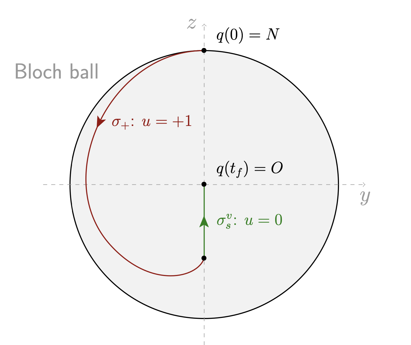
The time-minimal saturation problem is the following: starting from the North pole of the Bloch ball, the goal is to reach in minimum time the center of the Bloch ball, which corresponds at the final time to zero magnetization of the spin.

Time-minimal saturation problem

We define the time-minimal saturation problem as the following optimal control problem:

\[ \inf t_f, \quad \text{s.t.} \quad u(\cdot) \in \mathcal{U}, \quad t_f \ge 0 \quad \text{and} \quad q(t_f, N, u(\cdot)) = O,\]

where $N = (0, 1)$ is the North pole, where $O = (0,0)$ is the origin of the Bloch ball and where $t \mapsto q(t, q_0, u(\cdot))$ is the unique maximal solution of the 2D control system $\dot{q} = F_0(q) + u\, F_1(q)$ associated to the control $u(\cdot)$ and starting from the given initial condition $q_0$.

The inversion sequence ${\sigma_+} {\sigma_s^v}$, that is a positive bang arc followed by a singular vertical arc with zero control, is the simplest way to go from $N$ to $O$. Is it optimal?

We have the following symmetry.

Proposition. Let $(y(\cdot), z(\cdot))$, with associated control $u(\cdot)$, be a trajectory solution of $\dot{q} = F_0(q) + u\, F_1(q)$. Then, $(-y(\cdot), z(\cdot))$ with control $-u(\cdot)$ is also solution of this system.

This discrete symmetry allows us to consider only trajectories inside the domain $\{y \le 0\}$ of the Bloch ball.

In order to solve numerically the problem, we need to set the parameters. We introduce the practical cases in the following table. We give the relaxation times with the associated $(\gamma, \Gamma)$ parameters for $\omega_\mathrm{max} = 2 \pi\times 32.3$ Hz. Note that in the experiments, $\omega_\mathrm{max}$ may be chosen up to 15 000 Hz but we consider the same value as in ^[1].

Name	$T_1$	$T_2$	$\gamma$	$\Gamma$	$\delta=\gamma-\Gamma$
Water	2.5	2.5	$1.9710e^{-03}$	$1.9710e^{-03}$	$0.0$
Cerebrospinal Fluid	2.0	0.3	$2.4637e^{-03}$	$1.6425e^{-02}$	$-1.3961^{-02}$
Deoxygenated blood	1.35	0.05	$3.6499e^{-03}$	$9.8548e^{-02}$	$-9.4898^{-02}$
Oxygenated blood	1.35	0.2	$3.6499e^{-03}$	$2.4637e^{-02}$	$-2.0987^{-02}$
Gray cerebral matter	0.92	0.1	$5.3559e^{-03}$	$4.9274e^{-02}$	$-4.3918^{-02}$
White cerebral matter	0.78	0.09	$6.3172e^{-03}$	$5.4749e^{-02}$	$-4.8432^{-02}$
Fat	0.2	0.1	$2.4637e^{-02}$	$4.9274e^{-02}$	$-2.4637^{-02}$
Brain	1.062	0.052	$4.6397e^{-03}$	$9.4758e^{-02}$	$-9.0118^{-02}$
Parietal muscle	1.2	0.029	$4.1062e^{-03}$	$1.6991e^{-01}$	$-1.6580^{-02}$

Table: Matter name with associated relaxation times in seconds and relative $(\gamma, \Gamma)$ parameters with $\omega_\mathrm{max} = 2 \pi\times 32.3$ Hz and $u_\mathrm{max} = 1$.

Deoxygenated blood case

We consider the Deoxygenated blood case. According to Theorem 3.6 from ^[2] the optimal solution is of the form Bang-Singular-Bang-Singular (BSBS). The two bang arcs are with control $u=1$. The first singular arc is contained in the horizontal line $z=\gamma/2\delta$ while the second singular arc is contained in the vertical line $y=0$. We propose in the following to retrieve this result numerically.

Let us first define the parameters with the two vector fields $F_0$ and $F_1$.

import OptimalControl: ⋅
⋅(a::Number, b::Number) = a*b

# Blood case
T1 = 1.35 # s
T2 = 0.05

ω = 2π⋅32.3 # Hz
γ = 1/(ω⋅T1)
Γ = 1/(ω⋅T2)

δ = γ - Γ
zs = γ / 2δ # ordinate of the horizontal singular line

F0(y, z) = [-Γ⋅y, γ⋅(1-z)]
F1(y, z) = [-z, y]

q0 = [0, 1] # initial state: the North pole

Then, we can define the problem with OptimalControl.

using OptimalControl

ocp = @def begin

    tf ∈ R, variable
    t ∈ [0, tf ], time
    q = (y, z) ∈ R², state
    u ∈ R, control

    q(0)  == q0
    q(tf) == [0, 0]

    -1 ≤ u(t) ≤ 1

    q̇(t) == F0(q(t)...) + u(t) * F1(q(t)...)

    tf → min

    tf ≥ 0

end

Direct method

We start to solve the problem with a direct method. The problem is transcribed into a NLP optimization problem by OptimalControl. The NLP problem is then solved by the well-known solver Ipopt thanks to NLPModelsIpopt.

We first start with a coarse grid, with only 50 points. We provide an init to get a solution in the domain $y \le 0$.

using NLPModelsIpopt

N = 50
sol = solve(ocp; grid_size=N, init=(state=[-0.5, 0.0], ), print_level=4)

Total number of variables............................:      154
                     variables with only lower bounds:        1
                variables with lower and upper bounds:       51
                     variables with only upper bounds:        0
Total number of equality constraints.................:      104
Total number of inequality constraints...............:        0
        inequality constraints with only lower bounds:        0
   inequality constraints with lower and upper bounds:        0
        inequality constraints with only upper bounds:        0


Number of Iterations....: 69

                                   (scaled)                 (unscaled)
Objective...............:   4.3291584173530723e+01    4.3291584173530723e+01
Dual infeasibility......:   5.0955031860588917e-11    5.0955031860588917e-11
Constraint violation....:   1.7521539774634221e-12    1.7521539774634221e-12
Variable bound violation:   9.9810988363202569e-09    9.9810988363202569e-09
Complementarity.........:   2.2378427285538361e-11    2.2378427285538361e-11
Overall NLP error.......:   5.0955031860588917e-11    5.0955031860588917e-11


Number of objective function evaluations             = 85
Number of objective gradient evaluations             = 70
Number of equality constraint evaluations            = 85
Number of inequality constraint evaluations          = 0
Number of equality constraint Jacobian evaluations   = 70
Number of inequality constraint Jacobian evaluations = 0
Number of Lagrangian Hessian evaluations             = 69
Total seconds in IPOPT                               = 5.725

EXIT: Optimal Solution Found.

Then, we plot the solution thanks to Plots.

using Plots

plt = plot(sol; size=(700, 500), solution_label="(N = "*string(N)*")")

This rough approximation is then refine on a finer grid of 500 points. This two steps resolution increases the speed of convergence. Note that we provide the previous solution as initialisation.

N = 500
direct_sol = solve(ocp; grid_size=N, init=sol, print_level=4, tol=1e-12)

Total number of variables............................:     1504
                     variables with only lower bounds:        1
                variables with lower and upper bounds:      501
                     variables with only upper bounds:        0
Total number of equality constraints.................:     1004
Total number of inequality constraints...............:        0
        inequality constraints with only lower bounds:        0
   inequality constraints with lower and upper bounds:        0
        inequality constraints with only upper bounds:        0


Number of Iterations....: 11

                                   (scaled)                 (unscaled)
Objective...............:   4.2725098369300873e+01    4.2725098369300873e+01
Dual infeasibility......:   5.3823612233827589e-13    5.3823612233827589e-13
Constraint violation....:   2.4980018054066022e-16    2.4980018054066022e-16
Variable bound violation:   9.9941457332164418e-09    9.9941457332164418e-09
Complementarity.........:   5.0000793557472201e-13    5.0000793557472201e-13
Overall NLP error.......:   5.3823612233827589e-13    5.3823612233827589e-13


Number of objective function evaluations             = 12
Number of objective gradient evaluations             = 12
Number of equality constraint evaluations            = 12
Number of inequality constraint evaluations          = 0
Number of equality constraint Jacobian evaluations   = 12
Number of inequality constraint Jacobian evaluations = 0
Number of Lagrangian Hessian evaluations             = 11
Total seconds in IPOPT                               = 0.089

EXIT: Optimal Solution Found.

We can compare both solutions. The BSBS structure is revelead even if the second bang arc is not clearly demonstrated.

plot!(plt, direct_sol; solution_label="(N = "*string(N)*")")

We define a custom plot function to plot the solution inside the Bloch ball.

spin_plot — Function

Below, we plot again the solution but inside the Bloch ball. We can see that the first bang arc permits to reach the horizontal singular line $z=\gamma/2\delta$ which is depicted with a dashed line. The second bang arc is very short which explains why it is not well captured. We may refine the grid around this bang arc to capture it well but in the following we propose to use an indirect method to refine this approximation.

spin_plot(direct_sol; size=(700, 350))

To make the indirect method converge we need a good initial guess. We extract below the useful information from the direct solution to provide an initial guess for the indirect method. We need the initial costate together with the switching times between bang and singular arcs and the final time.

t  = time_grid(direct_sol)
q  = state(direct_sol)
p  = costate(direct_sol)
u  = control(direct_sol)
tf = variable(direct_sol)

t0 = 0
pz0 = p(t0)[2]

t_bang_1 = t[ (abs.(u.(t)) .≥ 0.25) .& (t .≤  5)]
t_bang_2 = t[ (abs.(u.(t)) .≥ 0.25) .& (t .≥ 35)]
t1 = max(t_bang_1...)
t2 = min(t_bang_2...)
t3 = max(t_bang_2...)

q1, p1 = q(t1), p(t1)
q2, p2 = q(t2), p(t2)
q3, p3 = q(t3), p(t3)

println("pz0 = ", pz0)
println("t1 = ", t1)
println("t2 = ", t2)
println("t3 = ", t3)
println("tf = ", tf)

pz0 = -10.134292900434756
t1 = 1.623553738033433
t2 = 36.23088341716714
t3 = 37.68353676172337
tf = 42.72509836930087

Indirect method

We introduce the pseudo-Hamiltonian

\[H(q, p, u) = H_0(q, p) + u\, H_1(q, p)\]

where $H_0(q, p) = p \cdot F_0(q)$ and $H_1(q, p) = p \cdot F_1(q)$ are both Hamiltonian lifts. According to the maximisation condition from the Pontryagin Maximum Principle (PMP), a bang arc occurs when $H_1$ is nonzero and of constant sign along the arc. On the contrary the singular arcs are contained in $H_1 = 0$. If $t \mapsto H_1(q(t), p(t)) = 0$ along an arc then its derivative is also zero. Thus, along a singular arc we have also

\[\frac{\mathrm{d}}{\mathrm{d}t} H_1(q(t), p(t)) = \{H_0, H_1\}(q(t), p(t)) = 0,\]

where $\{H_0, H_1\}$ is the Poisson bracket of $H_0$ and $H_1$.

Lie and Poisson brackets

Let $F_0$, $F_1$ be two smooth vector fields on a smooth manifold $M$ and $f$ a smooth function on $M$. Let $x$ be local coordinates. The Lie bracket of $F_0$ and $F_1$ is given by

\[ [F_0,F_1] \coloneqq F_0 \cdot F_1 - F_1 \cdot F_0,\]

with $(F_0 \cdot F_1)(x) = \mathrm{d} F_1(x) \cdot F_0(x)$. The Lie derivative $\mathcal{L}_{F_0} f$ of $f$ along $F_0$ is simply written $F_0\cdot f$. Denoting $H_0$, $H_1$ the Hamiltonian lifts of $F_0$, $F_1$, then the Poisson bracket of $H_0$ and $H_1$ is

\[ \{H_0,H_1\} \coloneqq \vec{H_0} \cdot H_1.\]

We also use the notation $H_{01}$ (resp. $F_{01}$) to write the bracket $\{H_0,H_1\}$ (resp. $[F_0,F_1]$) and so forth. Besides, since $H_0$, $H_1$ are Hamiltonian lifts, we have $\{H_0,H_1\}= p \cdot [F_0,F_1]$.

We define next a function to plot the switching function $t \mapsto H_1(q(t), p(t))$ and its derivative along the solution computed by the direct method.

switching_plot — Function

We can notice on the plots below that maximisation condition from the PMP is not satisfied. We can see that the switching function becomes negative along the first bang arc but there is no switching from the control plot. Besides, we can see that along the first singular arc, the switching function is not always zero.

H0 = Lift(q -> F0(q...))
H1 = Lift(q -> F1(q...))
H01  = @Lie { H0, H1 }

switching_plot(direct_sol, H1, H01; size=(700, 800))

We aim to compute a better approximation of the solution thanks to indirect shooting. To do so, we need to define the three different flows associated to the three different control laws in feedback form: bang control, singular control along the horizontal line and singular control along the vertical line.

Note

Let us recall that $\delta = \gamma - \Gamma$. Then, for any $q = (y,z)$ we have:

\[ \begin{aligned} F_{01}(q) &= -(\gamma - \delta z) \frac{\partial}{\partial y} + \delta y \frac{\partial}{\partial z}, \\[0.5em] F_{001}(q) &= \left( \gamma\, (\gamma - 2\Gamma) - \delta^2 z\right)\frac{\partial}{ \partial y} + \delta^2 y \frac{\partial}{\partial z}, \\[0.5em] F_{101}(q) &= 2 \delta y \frac{\partial}{\partial y} + (\gamma - 2 \delta z) \frac{\partial}{\partial z}. \end{aligned}\]

Along a singular arc, we have $H_1 = H_{01} = 0$, that is $p \cdot F_1 = p \cdot F_{01} = 0$. Since, $p$ is of dimension 2 and is nonzero, then we have $\det(F_1, F_{01}) = y ( \gamma - 2 \delta z) = 0$. This gives us the two singular lines.

Differentiating $t \mapsto H_1(q(t), p(t)) = 0$ a second time along a singular arc gives

\[ H_{001}(q(t), p(t)) + u(t)\, H_{101}(q(t), p(t)) = 0,\]

that is $p(t)$ is orthogonal to $F_{001}(q(t)) + u(t)\, F_{101}(q(t))$. Hence, the singular control is given by

\[ \det(F_1(q(t)), F_{001}(q(t))) + u(t) \, \det(F_1(q(t)), F_{101}(q(t))) = 0.\]

For $y=0$, $\det(F_1(q), F_{101}(q))$ is zero and thus the singular control is zero. We denote it $u_0 \coloneqq 0$. Along the horizontal singular line, that is for $z=\gamma/2\delta$, the control is given by

\[ u_s(y) \coloneqq \gamma (2\Gamma - \gamma) / (2 \delta y).\]

Note that we could have defined the singular control with the Hamiltonian lifts $H_{001}$ and $H_{101}$. See the Goddard tutorial for an example of such a computation.

using OrdinaryDiffEq

# Controls
u0 = 0                   # off control: vertical singular line
u1 = 1                   # positive bang control
us(y) = γ⋅(2Γ−γ)/(2δ⋅y)  # singular control: horizontal line

# Flows
tolerances = (abstol=1e-14, reltol=1e-10)

f0 = Flow(ocp, (q, p, tf) -> u0      ; tolerances...)
f1 = Flow(ocp, (q, p, tf) -> u1      ; tolerances...)
fs = Flow(ocp, (q, p, tf) -> us(q[1]); tolerances...)

With the previous flows, we can define the shooting function considering the sequence Bang-Singular-Bang-Singular. There are 3 switching times $t_1$, $t_2$ and $t_3$. The final time $t_f$ is unknown such as the initial costate. To reduce the sensitivy of the shooting function we also consider the states and costates at the switching times as unknowns and we add some matching conditions.

Note that the final time is free, hence, in the normal case, $H = -p^0 = 1$ along the solution of the PMP. Considering this condition at the initial time, we obtain $p_y(0) = -1$. At the entrance of the singular arcs, we must satisfy $H_1 = H_{01} = 0$. For the first singular arc, this leads to the conditions

\[ - p_y(t_1) z_s + p_z(t_1) y(t_1) = z(t_1) - z_s = 0.\]

At the entrance of the second singular arc, we have

\[ p_y(t_3) = y(t_3) = 0.\]

Finally, the solution has to satisfy the final condition $q(t_f) = (y(t_f), z(t_f)) = (0, 0)$. Since, the last singular arc is contained in $y=0$, the condition $y(t_f)=0$ is redundant and so we only need to check that $z(t_f) = 0$.

Altogether, this leads to the following shooting function.

function shoot!(s, pz0, t1, t2, t3, tf, q1, p1, q2, p2, q3, p3)

    p0 = [-1, pz0]

    q1_, p1_ = f1(t0, q0, p0, t1)
    q2_, p2_ = fs(t1, q1, p1, t2)
    q3_, p3_ = f1(t2, q2, p2, t3)
    qf , pf  = f0(t3, q3, p3, tf)

    s[1] = - p1[1] ⋅ zs + p1[2] ⋅ q1[1]   # H1 = H01 = 0 on the horizontal
    s[2] = q1[2] - zs                     # singular line, z=zs
    s[3] = p3[1]                          # H1 = H01 = 0 on the vertical
    s[4] = q3[1]                          # singular line, y=0
    s[5] = qf[2]                          # z(tf) = 0

    # matching conditions
    s[ 6: 7] = q1 - q1_
    s[ 8: 9] = p1 - p1_
    s[10:11] = q2 - q2_
    s[12:13] = p2 - p2_
    s[14:15] = q3 - q3_
    s[16:17] = p3 - p3_

end

We are now in position to solve the shooting equations. Due to the sensitivity of the first singular arc, we need to improve the initial guess obtained from the direct method to make the Newton solver converge. To do so, we set for the initial guess $z(t_1) = z_s$ and $p_z(t_1) = p_y(t_1) z_s / y(t_1)$.

We can see below from the norm of the shooting function that the initial guess is not very accurate.

# we refine the initial guess to make the Newton solver converge
q1[2] = zs
p1[2] = p1[1] ⋅ zs / q1[1]

# Norm of the shooting function at initial guess
using LinearAlgebra: norm

s = similar([pz0], 17)
shoot!(s, pz0, t1, t2, t3, tf, q1, p1, q2, p2, q3, p3)

println("Norm of the shooting function: ‖s‖ = ", norm(s), "\n")

Norm of the shooting function: ‖s‖ = 229.6219709014965

Finally, we can solve the shooting equations thanks to NonlinearSolve and improve our solution.

using NonlinearSolve

# auxiliary function with aggregated inputs
nle = (s, ξ, λ) -> shoot!(s, ξ[1], ξ[2:5]..., ξ[6:7], ξ[8:9],
                            ξ[10:11], ξ[12:13], ξ[14:15], ξ[16:17])

# initial guess
ξ = [ pz0 ; t1 ; t2 ; t3 ; tf ; q1 ; p1 ; q2 ; p2 ; q3 ; p3]

# NLE problem
prob = NonlinearProblem(nle, ξ)

# resolution of S=0
indirect_sol = NonlinearSolve.solve(prob, SimpleNewtonRaphson(); abstol=1e-8, reltol=1e-8, show_trace=Val(true))

# we retrieve the costate solution together with the times
pz0 = indirect_sol.u[1]
t1 = indirect_sol.u[2]
t2 = indirect_sol.u[3]
t3 = indirect_sol.u[4]
tf = indirect_sol.u[5]
q1 = indirect_sol.u[6:7]
p1 = indirect_sol.u[8:9]
q2 = indirect_sol.u[10:11]
p2 = indirect_sol.u[12:13]
q3 = indirect_sol.u[14:15]
p3 = indirect_sol.u[16:17]

println("pz0 = ", pz0)
println("t1 = ", t1)
println("t2 = ", t2)
println("t3 = ", t3)
println("tf = ", tf)

# Norm of the shooting function at solution
s = similar([pz0], 17)
shoot!(s, pz0, t1, t2, t3, tf, q1, p1, q2, p2, q3, p3)
println("Norm of the shooting function: ‖s‖ = ", norm(s), "\n")

pz0 = -10.10302716212744
t1 = 1.6450509469601813
t2 = 37.32398129098127
t3 = 37.58077358002954
tf = 42.71370875364003
Norm of the shooting function: ‖s‖ = 6.26345902287027e-12

Let us plot the solution from the indirect method. We can notice that the second bang arc is well captured by the indirect method compared to the direct method.

# concatenation of the flows with the switching times
f = f1 * (t1, fs) * (t2, f1) * (t3, f0)

# computation of the solution: state, costate, control
indirect_sol = f((t0, tf), q0, [-1, pz0])

# plot in the Bloch ball
spin_plot(indirect_sol; size=(700, 350))

From the following plot, we can conclude that the maximisation condition from the PMP is now well satisfied compared to the solution obtained from the direct method.

switching_plot(indirect_sol, H1, H01; size=(700, 800))

1B. Bonnard, O. Cots, S. Glaser, M. Lapert, D. Sugny & Y. Zhang, *Geometric optimal control of the contrast imaging problem in nuclear magnetic resonance, IEEE Trans. Automat. Control, 57 (2012), no. 8, 1957–1969.
2Bonnard, B.; Cots, O.; Rouot, J.; Verron, T. Time minimal saturation of a pair of spins and application in magnetic resonance imaging. Mathematical Control and Related Fields, 2020, 10 (1), pp.47-88. https://inria.hal.science/hal-01779377