Switching structure

An indirect method fixes the structure of the solution: the times at which the control law changes, the jumps of the state or costate at these times, the sequence of arcs (bang, singular, boundary, …). A direct method does not: it returns values on a grid. A Solution keeps this structure in a SwitchingModel, given to build_solution with the switching keyword:

• the switching times, strictly inside the time span;

• one label per phase ("" for a phase with no label);

• the left and right limits of the state, costate and control at every switching time;

• optionally, the left and right limits of the duals, by label (duals), when a multiplier jumps at a junction: path constraints and state or control boxes.

The trajectories of the solution stay single-valued and left-continuous: at a switching time, state(sol)(tᵢ) returns the value before the jump. The value after it is read with right_limit.

A solution with a jump

The state below jumps by +1 at t = 0.5, where the control switches from 1 to -1:

using CTModels

pre = CTModels.PreModel()
CTModels.time!(pre; t0=0.0, tf=1.0)
CTModels.state!(pre, 1)
CTModels.control!(pre, 1)
CTModels.dynamics!(pre, (r, t, x, u, v) -> (r[1] = u; nothing))
CTModels.objective!(pre, :min; lagrange=(t, x, u, v) -> 0.5 * u^2)
CTModels.time_dependence!(pre; autonomous=true)
ocp = CTModels.build(pre)

τ = 0.5
T = collect(range(0.0, 1.0; length=11))
X = reshape([t <= τ ? t : t + 1 for t in T], :, 1)
U = reshape([t <= τ ? 1.0 : -1.0 for t in T], :, 1)
P = zeros(length(T), 1)

switching = CTModels.SwitchingModel(;
    times=[τ],
    labels=["bang+", "bang-"],
    state=([τ;;], [τ + 1;;]),        # (left, right), one row per switching time
    costate=([0.0;;], [0.0;;]),
    control=([1.0;;], [-1.0;;]),
)
sol = CTModels.build_solution(ocp, T, X, U, Float64[], P;
    objective=0.0, successful=true, control_interpolation=:linear, switching=switching)

Solution  ✓ successful
  │  Objective : 0.0
  │  Switching times : [0.5]
  └─ Phases : bang+ → bang-

The display lists the switching times and the sequence of phases; an unlabelled phase shows as ·.

Reading the structure

julia> CTModels.switching_times(sol)
1-element Vector{Float64}:
 0.5

julia> CTModels.phase_labels(sol)
2-element Vector{String}:
 "bang+"
 "bang-"

julia> CTModels.state(sol)(τ)                    # left-continuous: before the jump
0.5

julia> CTModels.right_limit(sol, :state, 1)      # after the jump
1.5

julia> CTModels.left_limit(sol, :control, 1), CTModels.right_limit(sol, :control, 1)
(1.0, -1.0)

A one-dimensional component is a scalar, as everywhere in CTModels.

When the trajectories are given as matrices, the interpolation uses the limits, so that the jump is not smeared over the grid cell that follows it:

julia> CTModels.state(sol)(0.55)                 # between the right limit 1.5 and x(0.6) = 1.6
1.55

Trajectories given as functions are used as they are.

Plotting

Each jump is drawn as a vertical segment, from the left to the right limit; a vertical line marks each switching time, with the look of the initial and final time markers; the phase labels are written on the control cell:

plot(sol)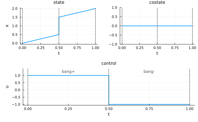

Keyword	Values (default first)	Effect
switching_style	NamedTuple() / a NamedTuple / :none	style of the switching-time lines, merged on the time markers' style; :none hides them
phase_labels	:control / :all / :none	write the labels on the control cell (or on the first drawn group when the control is not drawn), on every group, or nowhere
phase_labels_style	NamedTuple()	color, fontsize, halign, valign of the labels
jumps	:segment / :none	draw a jump as a vertical segment, or break the curve between the two limits

plot(sol; switching_style=(color=:red,), phase_labels=:all)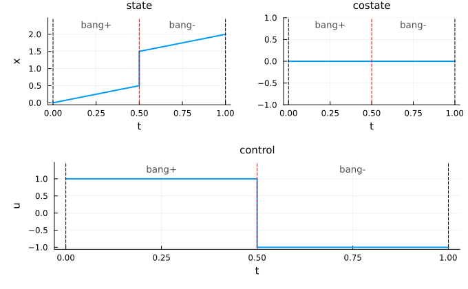

The vertical segment makes a jump easy to see, and to compare with a solution whose jump is smoothed, e.g. from a direct method. It does not mean that the trajectory takes the values in between: with jumps=:none, the curve stops at the left limit and starts again at the right limit.

plot(sol; jumps=:none)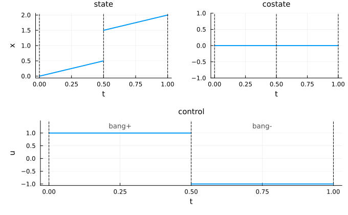

The whole trajectory keeps one color: the phases are parts of the same curve, not separate series. A solution drawn on top with plot! takes the next color, as usual.

Duals of the path constraints

A multiplier usually jumps at the entry and the exit of a boundary arc (0 on an interior arc, positive on the boundary arc). When the limits of the duals are given (by label, in duals), the dual panel draws the jump as the other panels do. The solution of a flow of CTFlows fills them.

pre = CTModels.PreModel()
CTModels.time!(pre; t0=0.0, tf=1.0)
CTModels.state!(pre, 1)
CTModels.control!(pre, 1)
CTModels.dynamics!(pre, (r, t, x, u, v) -> (r[1] = u; nothing))
CTModels.objective!(pre, :min; lagrange=(t, x, u, v) -> 0.5 * u^2)
CTModels.constraint!(pre, :path; f=(r, t, x, u, v) -> (r[1] = x; nothing),
    lb=0.0, ub=Inf, label=:xmin)
CTModels.time_dependence!(pre; autonomous=true)
ocp_c = CTModels.build(pre)

X = reshape([t <= τ ? 0.5 - t : 0.0 for t in T], :, 1)   # x reaches 0 at τ, then stays
U = reshape([t <= τ ? -1.0 : 0.0 for t in T], :, 1)
switching = CTModels.SwitchingModel(;
    times=[τ],
    labels=["interior", "boundary"],
    state=([0.0;;], [0.0;;]),
    costate=([0.0;;], [0.0;;]),
    control=([-1.0;;], [0.0;;]),
    duals=Dict(:xmin => ([0.0], [1.0])),    # μ = 0, then 1 on the boundary arc
)
sol_c = CTModels.build_solution(ocp_c, T, X, U, Float64[], P;
    objective=0.0, successful=true, switching=switching,
    duals=Dict(:xmin => t -> t <= τ ? 0.0 : 1.0))
plot(sol_c, :state, :control, :path, :dual)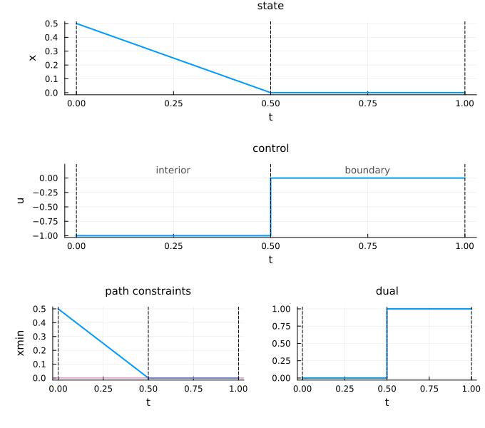

Limits of the duals by label

A switching model is built without the model, so it cannot know where the rows of a label are. It keeps the limits given in duals by label, and build_solution places them on the layout of the model (see How the duals are stored):

Label	label => (left, right)	Stored in
path constraint	one row per switching time, one column per row of the label	limits(sw, :path_dual), one column per row of the stacked path constraint
state box	the signed dual (what dual returns), one column per component of the label	limits(sw, :state_dual), one column per state component
control box	the same	limits(sw, :control_dual), one column per control component

A vector stands for a one-row label. In a kind where some labels are given, the columns of the others are NaN; a kind with no label keeps no column (limits not known). Boundary and variable labels take no limits: their duals do not depend on time.

julia> sw_d = CTModels.SwitchingModel(; times=[τ], duals=Dict(:xmin => ([0.0], [1.0])));

julia> sol_d = CTModels.build_solution(ocp_c, T, X, U, Float64[], P;
           objective=0.0, successful=true, switching=sw_d,
           duals=Dict(:xmin => t -> t <= τ ? 0.0 : 1.0));

julia> CTModels.Solutions.limits(CTModels.switching_model(sol_d), :path_dual)
([0.0;;], [1.0;;])

Deprecated: path_dual

SwitchingModel(; path_dual=(left, right)) gave the limits of the stacked path duals by position, one column per row of the path constraint. It still works, with a deprecation warning, and will be removed at the next breaking release; give the limits by label in duals.

The limits of the box duals are stored and saved, but not drawn yet: the box duals get their own rows in the plot with CTModels.jl#506.

Saving and loading

export_ocp_solution writes the switching structure with the solution (JLD2 and JSON), and import_ocp_solution reads it back, so the imported trajectories keep their jumps. A file without switching structure, including a file written by an older version, is read with an EmptySwitchingModel.

Time grids have no repeated time

A trajectory takes one value at each time: a time grid with a repeated time raises an IncorrectArgument. A jump is stored in the switching model, not as a repeated time with two values.

julia> CTModels.build_solution(ocp, [0.0, 0.5, 0.5, 1.0], zeros(4, 1), zeros(4, 1), Float64[],
           zeros(4, 1); objective=0.0, successful=true)
ERROR: IncorrectArgument
│
│  repeated time in the state time grid
│
│  Got       time 0.5 appears more than once
│  Expected  a strictly increasing time grid (each time once)
│
│  Context   build_solution - validating the state time grid
│  Hint      Keep each time once. To store a jump at a switching time, give the left and right limits in `switching=SwitchingModel(...)`.
└─